

Chapter 9: Markov Chain Monte Carlo#
Key Takeaway#
Jump to Section 9.6

Intro#
If you’ve ever wondered how probabilistic programming packages like PyMC ever generated samples of a posterior distribution based on the priors you specified in the model, along with the data, it turns out that the machine driving this stochastic process is known as Markov Chain Monte Carlo. We mentioned this sampling technique as early as chapter 2 and 4, as one of the conditioning engines that could be used to sample directly estimate models, such as the Generalized Linear Model or Multi-Level models which routinely produce non-Gaussian posterior distributions. However unlike techniques like grid approximation which doesn’t scale, or quadratic approximation which assumes the posterior always resembles a Gaussian shape, Markov Chain Monte Carlo can sample directly from the posterior directly without assuming a shape at a fraction of the computation associated to grid approximation.
Rethinking: Stan the man.#
The Stan programming language was actually named after Stanislaw Ulam (1909–1984) who was credited as one of the inventors of the Markov Chain Monte Carlo. Together with Ed Teller, Stan applied their invention to the design of the fusion bomb along with other diverse problems of less monstrous nature after the war such as in the fields of pure mathematics, statistical physics, chaos theory, and molecular and theoretical biology.
import warnings

import arviz as az
import matplotlib.pyplot as plt
import matplotlib.patheffects as pe
import matplotlib.patches as mpatches
import numpy as np
import pandas as pd
import pymc as pm
import warnings

from matplotlib.gridspec import GridSpec
from matplotlib.colors import LinearSegmentedColormap
from scipy import stats
from scipy.stats import multivariate_normal
from scipy.ndimage import gaussian_filter

warnings.simplefilter(action="ignore", category=FutureWarning)
pd.set_option("mode.chained_assignment", None)
%config Inline.figure_format = 'retina'
az.style.use("arviz-darkgrid")
az.rcParams["stats.hdi_prob"] = 0.89  # sets default credible interval used by arviz
Section 9.1 - Good King Markov and His island kingdom.#
Code 9.1#
##########################
### OLD EXPLAINER CODE ###
##########################
num_weeks = int(100000)
positions = np.zeros(num_weeks)
current = 10

for i in range(num_weeks):
    # record current position
    positions[i] = current

    # flip coin to generate proposal
    proposal = current + np.random.choice([-1, 1])
    # loop around the archipelago
    if proposal < 1:
        proposal = 10
    if proposal > 10:
        proposal = 1

    # move?
    prob_move = proposal / current
    if np.random.uniform() < prob_move:
        current = proposal
Code 9.2 & 9.3#
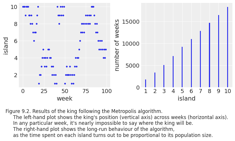
# Figure 9.2
_, axs = plt.subplots(1, 2, figsize=[8, 3.5], constrained_layout=True)

ax0, ax1 = axs

nplot = 100
ax0.scatter(range(nplot), positions[:nplot], s=10)
ax0.set_ylabel("island")
ax0.set_xlabel("week")

counts, _ = np.histogram(positions, bins=10)
ax1.bar(range(10), counts, width=0.1)
ax1.set_ylabel("number of weeks")
ax1.set_xlabel("island")
ax1.set_xticks(range(10))
ax1.set_xticklabels(range(1, 11))

#####################
### CODE ADDITION ###
#####################
plt.suptitle(
    x=0.5,
    y=-0.06,
    t="Figure 9.2. Results of the king following the Metropolis algorithm. \n \
    The left-hand plot shows the king's position (vertical axis) across weeks (horizontal axis). \n \
    In any particular week, it's nearly impossible to say where the king will be. \n \
    The right-hand plot shows the long-run behaviour of the algorithm, \n \
    as the time spent on each island turns out to be proportional to its population size.",
    ma="left"
  );
Explaining Markov Chain Monte Carlo (MCMC) with Prof Markov and the burnt forest#
Prof. Markov is a wildfire forensic ecologist working for the BC Wildfire Service assigned to investigate a remote section of the Cathedral Grove forest on Vancouver Island that burned overnight. By morning, helicopters have marked the burn scar which are identified as the cells that are completely black on a 5x5 grid map (i.e. 25 total cells), along with the cells that are untouched and green. The pattern of char intensity and fire spread direction leaves a forensic signature pointing toward where the fire originated.
Prof. Markov’s job is to estimate the location of the ignition source of the fire but unfortunately he can’t just walk to it. The terrain is rugged, some areas are still smoldering, and even the best forensic evidence leaves genuine ambiguity because wind shifts, overlapping fuel beds, and spotting prevents the true ignition location from ever being known with certainty. Essentially, a single point estimate (i.e. “the fire started here”) in this case would be scientifically dishonest. What he needs is a probability distribution over the entire grid which would quantify which cells are potential ignition sources and how plausible is each one relative to the others.
However, Prof. Markov has two sources of information.
The first is a prior which are historical records that describe which cells/areas carry a higher baseline ignition risk before he’s examined a single tree. These historical records quantify risk based on factors such as the proximity to logging roads, known campfire sites, or dry lightning strike frequency.
The second source of information is a likelihood which is the burn pattern of the fire itself. Cells that sit at the upwind origin of the spread, surrounded by the most intense char, and with fire vectors radiating outward, score higher as candidate ignition sources.
For each of the 25 cells in the grid, Prof. Markov computes the unnormalised posterior by simply multiplying the prior ignition risk of that cell by the likelihood score given the observed burn pattern. This gives him a grid of 25 positive values stored in the example_posterior_dist object where higher values indicate more plausible ignition sources. Note that these values don’t need to sum to 1 since they’re supposed to be unnormalised. Therefore, Markov’s posterior represents the thing that he actually wants which combines both the prior and the likelihood:
Which is essentially Bayes’ Theorem at its core:
To turn our posterior, \(P( H \mid E)\), into a proper probability distribution, Markov would need to compute the total probability mass across every cell in the grid, summing the right-hand side over all 25 cells, then dividing by that sum. Over the real Cathedral Grove landscape with millions of candidate ignition points, doing this math is completely impractical as he would never be able to write it down, let alone compute it.
This method is basically the one used for grid approximation but luckily, there’s smarter ways to solve this problem of sampling from the posterior. Here’s how it works:
Prof. Markov moves through the grid one cell at a time, collecting forensic evidence as he goes. Each day he follows these three rules:
1. Roll an eight-sided die (i.e. an octahedron dice) to propose a move in one of the following directions: 1 = North, 2 = Northeast, 3 = East, 4 = Southeast, 5 = South, 6 = Southwest, 7 = West, or 8 = Northwest. If the roll would take him outside the grid, re-roll until it doesn’t.
2. Evaluate the posterior probability of the proposed cell (\(p_{\text{move}}\)) relative to his current position: $\(p_{\text{move}} = \frac{P(\text{ignition at proposed cell} \mid \text{burn pattern})}{P(\text{ignition at current position} \mid \text{burn pattern})}\)$
3. If \(p_{\text{move}} \geq 1\), that means the proposed cell is more probable than the current one so he should move there with certainty. If \(p_{\text{move}} < 1\), this means that the proposed cell is less probable than the current one. In this case, Prof. Markov then needs to draw a random number (\(u\)) from a uniform random number generator between 0 and 1.
If \(u < p_{\text{move}}\), then he can move to the proposed cell. But if \(u \geq p_{\text{move}}\), then he needs stay put. The lower the ratio, the more likely the draw fails which therefore means he must stays put.
With Python code, let’s examine how this algorithm works when Prof. Markov works through num_days = 10 different cells:
example_posterior_dist = np.array([
    [1.2,  2.1,  3.4,  2.8,  1.5],
    [1.8,  4.2,  7.1,  5.3,  2.3],
    [2.5,  6.8, 10.0,  8.4,  3.7],
    [1.9,  5.1,  8.6,  6.9,  4.2],
    [1.1,  2.7,  4.3,  3.5,  2.0],
])

print("Ignition Source Posterior Probabilities Grid:")
print(example_posterior_dist)

##########################
### Metropolis Sampler ###
##########################
D8_MOVES = [
    (-1,  0),   # North
    (-1, +1),   # Northeast
    ( 0, +1),   # East
    (+1, +1),   # Southeast
    (+1,  0),   # South
    (+1, -1),   # Southwest
    ( 0, -1),   # West
    (-1, -1),   # Northwest
]

D8_NAMES = ["North", "Northeast", "East", "Southeast", "South", "Southwest", "West", "Northwest"]

num_days = 10 # int(100000)
positions = []
current   = (0, 0)        # start at top-left corner of the grid

for day in range(num_days):
    # record current position
    positions.append(current)

    # Rule 1 — Roll D8 and re-roll if outside the grid
    # roll D8 to generate proposal
    roll = np.random.randint(8)
    dr, dc = D8_MOVES[roll]
    direction = D8_NAMES[roll]

    proposal = (current[0] + dr, current[1] + dc)

    # re-roll if proposal falls outside the grid
    while not (0 <= proposal[0] < 5 and 0 <= proposal[1] < 5):
      roll = np.random.randint(8)
      dr, dc = D8_MOVES[roll]
      direction = D8_NAMES[roll]

      proposal = (current[0] + dr, current[1] + dc)

    print(f"\nDay {day + 1}")
    print(f"Current position: {current}  (posterior = {example_posterior_dist[current]:.1f})")
    print(f"[Rule 1] Rolled: {direction} → proposed {proposal}  (posterior = {example_posterior_dist[proposal]:.1f})")

    # Rule 2 — Compute the acceptance ratio:
    # move?
    prob_move = example_posterior_dist[proposal] / example_posterior_dist[current]
    print(f"[Rule 2] Acceptance ratio : {example_posterior_dist[proposal]:.3f} / {example_posterior_dist[current]:.3f} = {prob_move:.3f}")

    # Rule 3 — Move or stay put:
    # this will always be >1 (outside of np.random.uniform())if proposal is greater
    # if np.random.uniform() < prob_move:
    #   current = proposal

    # Rule 3 — Move or stay put:
    if prob_move >= 1:
        current = proposal
        print(f"[Rule 3] Decision: p_move >= 1 — moved to {current} without hesitation")
    else:
        u = np.random.uniform()
        if u < prob_move:
            current = proposal
            print(f"Decision: p_move < 1 — drew u = {u:.3f} < {prob_move:.3f} — moved to {current}")
        else:
            print(f"Decision: p_move < 1 — drew u = {u:.3f} >= {prob_move:.3f} — staying put at {current}")
Ignition Source Posterior Probabilities Grid:
[[ 1.2  2.1  3.4  2.8  1.5]
 [ 1.8  4.2  7.1  5.3  2.3]
 [ 2.5  6.8 10.   8.4  3.7]
 [ 1.9  5.1  8.6  6.9  4.2]
 [ 1.1  2.7  4.3  3.5  2. ]]

Day 1
Current position: (0, 0)  (posterior = 1.2)
[Rule 1] Rolled: South → proposed (1, 0)  (posterior = 1.8)
[Rule 2] Acceptance ratio : 1.800 / 1.200 = 1.500
[Rule 3] Decision: p_move >= 1 — moved to (1, 0) without hesitation

Day 2
Current position: (1, 0)  (posterior = 1.8)
[Rule 1] Rolled: North → proposed (0, 0)  (posterior = 1.2)
[Rule 2] Acceptance ratio : 1.200 / 1.800 = 0.667
Decision: p_move < 1 — drew u = 0.643 < 0.667 — moved to (0, 0)

Day 3
Current position: (0, 0)  (posterior = 1.2)
[Rule 1] Rolled: South → proposed (1, 0)  (posterior = 1.8)
[Rule 2] Acceptance ratio : 1.800 / 1.200 = 1.500
[Rule 3] Decision: p_move >= 1 — moved to (1, 0) without hesitation

Day 4
Current position: (1, 0)  (posterior = 1.8)
[Rule 1] Rolled: Southeast → proposed (2, 1)  (posterior = 6.8)
[Rule 2] Acceptance ratio : 6.800 / 1.800 = 3.778
[Rule 3] Decision: p_move >= 1 — moved to (2, 1) without hesitation

Day 5
Current position: (2, 1)  (posterior = 6.8)
[Rule 1] Rolled: West → proposed (2, 0)  (posterior = 2.5)
[Rule 2] Acceptance ratio : 2.500 / 6.800 = 0.368
Decision: p_move < 1 — drew u = 0.525 >= 0.368 — staying put at (2, 1)

Day 6
Current position: (2, 1)  (posterior = 6.8)
[Rule 1] Rolled: East → proposed (2, 2)  (posterior = 10.0)
[Rule 2] Acceptance ratio : 10.000 / 6.800 = 1.471
[Rule 3] Decision: p_move >= 1 — moved to (2, 2) without hesitation

Day 7
Current position: (2, 2)  (posterior = 10.0)
[Rule 1] Rolled: Northeast → proposed (1, 3)  (posterior = 5.3)
[Rule 2] Acceptance ratio : 5.300 / 10.000 = 0.530
Decision: p_move < 1 — drew u = 0.447 < 0.530 — moved to (1, 3)

Day 8
Current position: (1, 3)  (posterior = 5.3)
[Rule 1] Rolled: Northwest → proposed (0, 2)  (posterior = 3.4)
[Rule 2] Acceptance ratio : 3.400 / 5.300 = 0.642
Decision: p_move < 1 — drew u = 0.636 < 0.642 — moved to (0, 2)

Day 9
Current position: (0, 2)  (posterior = 3.4)
[Rule 1] Rolled: Southwest → proposed (1, 1)  (posterior = 4.2)
[Rule 2] Acceptance ratio : 4.200 / 3.400 = 1.235
[Rule 3] Decision: p_move >= 1 — moved to (1, 1) without hesitation

Day 10
Current position: (1, 1)  (posterior = 4.2)
[Rule 1] Rolled: Northeast → proposed (0, 2)  (posterior = 3.4)
[Rule 2] Acceptance ratio : 3.400 / 4.200 = 0.810
Decision: p_move < 1 — drew u = 0.944 >= 0.810 — staying put at (1, 1)
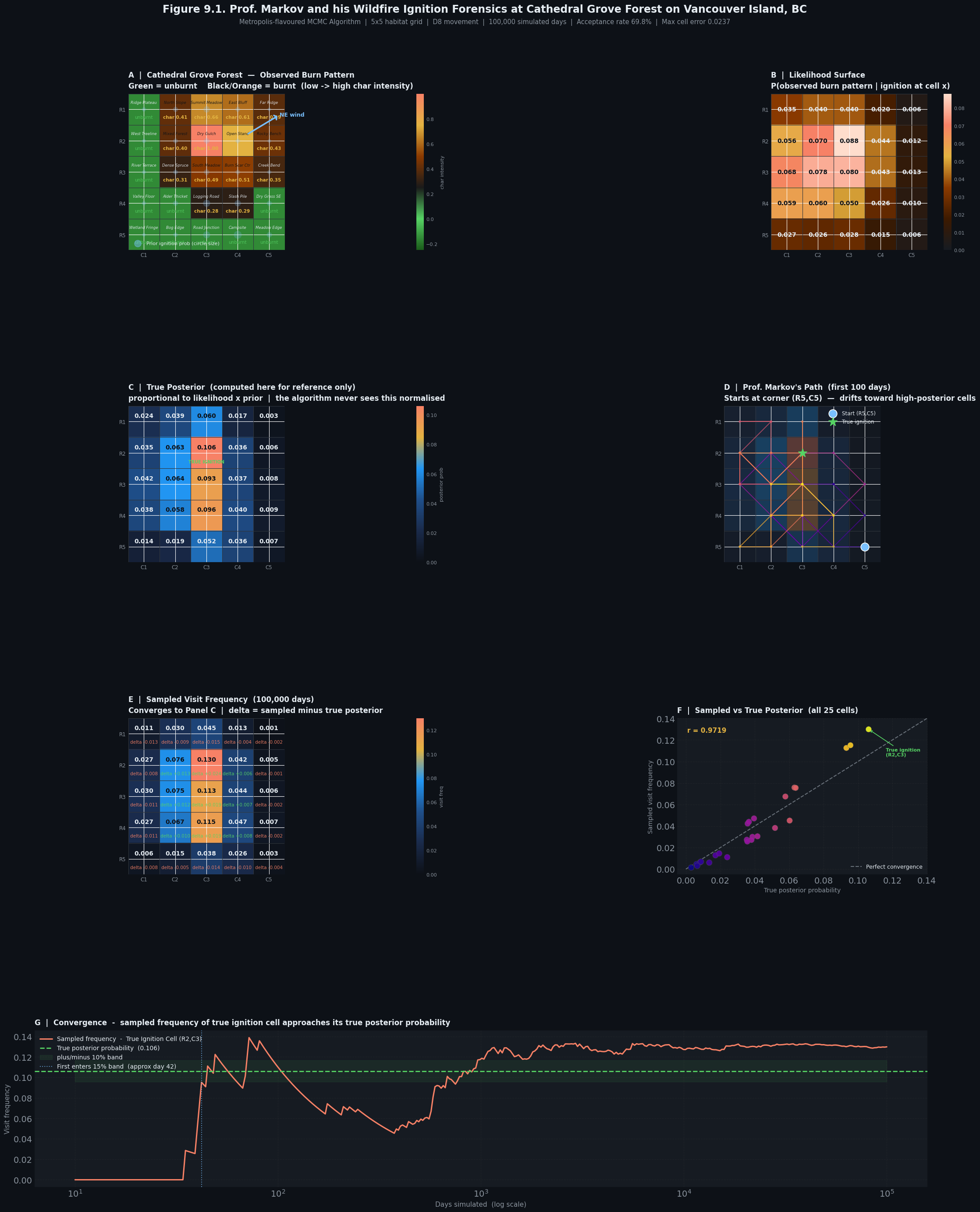
After enough days of traversing the grid this way, the proportion of time Prof. Markov spends in each cell converges to that cell’s true posterior probability. He’ll visit high-probability ignition cells most often and low-probability cells less often, not because he was told their probabilities in advance, but because the accept/reject rule steers him there naturally over time. Panel D of the figure below shows his path across the first 100 steps, starting in the sparse top-left corner and gradually drifting toward the high-posterior central cells.
Panel E shows visit frequencies after 100,000 steps where the sampler has tightly recovered the true posterior distribution across all 25 cells. One thing to note about Panel E titled “Sampled Visit Frequency” is that this graph essentially equivalent to the one-dimensional posterior distirbution histogram that we typically generate whenever we build a Bayesian model. The reason why we don’t have that same histogram where we typically use the ax.plot_density() function to generate is because in our case, each cell that we sampled is a two-dimensional object. Although we can, in theory, “flatten” the X and Y coordinates in order to build a histogram that counted up how much each cell was sampled, it wouldn’t be as effective of a visualization due to the categorical nature of the cells which is why a heatmap for this panel made more sense in this situation. In structuring our example this way, we’re then able to emphasize the idea that a posterior distribution doesn’t have to be just a bell curve on a historgram. A posterior can also be a 25-element probability mass function spread across a spatial grid.
Panel G shows the Monte Carlo payoff which we can define as the cumulative visit frequency of the peak cell, locking onto its true posterior probability as the run lengthens. This last point is worth dwelling on. Markov doesn’t just want to know which single cell is most likely. That would be a point estimate which is no better than a guess. He wants to know the full distribution which represents how confident can he be in the top candidate of the ignition source, how much probability mass sits in the neighbouring cells, and which regions of the grid can be ruled out entirely. The record of positions he accumulates over 100,000 days is that distribution. Every quantity of forensic interest — the probability that the ignition source was within 100 metres of the logging road, the 89% credible region of candidate cells, the expected char intensity at the true ignition point — can be estimated simply by averaging over that record. That is the Monte Carlo part of Markov Chain Monte Carlo.
The approach Prof. Markov is using is the Metropolis algorithm flavour, the oldest and simplest member of the MCMC family. Its power comes from one profound property: That it works in spaces where exhaustive enumeration is impossible. But over a real continuous landscape, the number of candidate ignition points is infinite. There is no grid to sum over, no list of cells to evaluate. However, the algorithm doesn’t need a list. It only ever asks one question at a time: Is where I might go more or less probable than where I am right now? That local comparison, repeated thousands of times, is enough to map out the entire posterior distribution and it requires nothing from the intractable normalising constant that would otherwise make the problem unsolvable.
Rethinking: Why the normalizing constant doesn’t matter#
If we look closely at the acceptance ratio in step 2, we’ll realize that the normalizing constant doesn’t matter. The posterior of each cell is proportional to likelihood × prior. When you divide one cell’s posterior by another’s, the normalising constant (i.e. the intractable sum over all cells) appears in both the numerator and denominator which therefore cancels out exactly:
\(p_{\text{move}} = \frac{P(\text{proposed} \mid \text{data})}{P(\text{current} \mid \text{data})} \)
\(p_{\text{move}} = \frac{\overbrace{P(\text{data} \mid \text{proposed}) \times P(\text{proposed})}^{\text{unnormalised posterior}} / Z}{\underbrace{P(\text{data} \mid \text{current}) \times P(\text{current})}_{\text{unnormalised posterior}} / Z}\)
\(p_{\text{move}} = \frac{P(\text{data} \mid \text{proposed}) \times P(\text{proposed})}{P(\text{data} \mid \text{current}) \times P(\text{current})}\)
where \(Z\) is the normalising constant. Prof. Markov never needs to know it. He only ever needs to evaluate the unnormalised posterior at two points: Where he is now and where he might go next, then compute their ratio. That ratio is all the algorithm needs to make a valid decision.
Figure 9.1. & 9.2. Prof. Markov and his Wildfire Ignition Forensics at Cathedral Grove Forest on Vancouver Island, BC#
rng = np.random.default_rng(137)

TRUE_IGNITION = (1, 2)

cell_names = [
    ["Ridge Plateau",  "North Slope",   "Summit Meadow", "East Bluff",    "Far Ridge"],
    ["West Treeline",  "Mixed Forest",  "Dry Gulch",     "Open Stand",    "Rocky Bench"],
    ["River Terrace",  "Dense Spruce",  "South Meadow",  "Burn Scar Ctr", "Creek Bend"],
    ["Valley Floor",   "Alder Thicket", "Logging Road",  "Slash Pile",    "Dry Grass SE"],
    ["Wetland Fringe", "Bog Edge",      "Road Junction", "Campsite",      "Meadow Edge"],
]

# --- PRIOR ---
prior_raw = np.array([
    [0.6, 0.7, 1.8, 0.6, 0.4],
    [0.5, 0.8, 1.2, 0.7, 0.4],
    [0.5, 0.6, 0.9, 0.6, 0.5],
    [0.6, 0.7, 2.5, 1.1, 0.8],
    [0.4, 0.4, 1.6, 2.8, 0.6],
], dtype=float)
prior_raw = gaussian_filter(prior_raw, sigma=0.6)
prior = prior_raw / prior_raw.sum()

# --- BURN PATTERN ---
WIND_DR = np.array([-0.3, 0.6])
char_intensity = np.zeros((5, 5))
for r in range(5):
    for c in range(5):
        vec = np.array([r - TRUE_IGNITION[0], c - TRUE_IGNITION[1]], dtype=float)
        dist = np.linalg.norm(vec) + 1e-6
        wind_align = np.dot(vec, WIND_DR) / dist
        char_intensity[r, c] = np.exp(-0.55 * dist) * (1.0 + 0.5 * wind_align)
char_intensity = np.clip(char_intensity, 0.01, None)
BURN_THRESHOLD = 0.28
burnt = char_intensity > BURN_THRESHOLD

# --- LIKELIHOOD ---
burnt_coords = np.argwhere(burnt)
centroid = burnt_coords.mean(axis=0)

likelihood_raw = np.zeros((5, 5))
for r in range(5):
    for c in range(5):
        dist_centroid = np.linalg.norm(np.array([r, c]) - centroid)
        centroid_score = np.exp(-0.7 * dist_centroid)
        vec_from_cent = np.array([r - centroid[0], c - centroid[1]])
        upwind_score = np.exp(-1.2 * np.dot(vec_from_cent, WIND_DR))
        char_score = char_intensity[r, c] ** 0.5
        burnable_penalty = 0.5 if r == 4 and c in [0, 1] else 1.0
        likelihood_raw[r, c] = centroid_score * upwind_score * char_score * burnable_penalty

likelihood_raw = gaussian_filter(likelihood_raw, sigma=0.5)
likelihood_raw = np.clip(likelihood_raw, 1e-4, None)
likelihood = likelihood_raw / likelihood_raw.sum()

# --- POSTERIOR ---
posterior_unnorm = likelihood_raw * prior_raw
posterior = posterior_unnorm / posterior_unnorm.sum()

# --- SAMPLER ---
D8_MOVES = [(-1,0),(-1,1),(0,1),(1,1),(1,0),(1,-1),(0,-1),(-1,-1)]
num_days = int(100000)
board_positions = []
current = (4, 4)
accepted = 0
trace_full = []

for day in range(num_days):
    board_positions.append(current)
    trace_full.append(current)
    roll = rng.integers(0, 8)
    dr, dc = D8_MOVES[roll]
    nr, nc = current[0] + dr, current[1] + dc
    attempts = 0
    while not (0 <= nr < 5 and 0 <= nc < 5):
        roll = rng.integers(0, 8)
        dr, dc = D8_MOVES[roll]
        nr, nc = current[0] + dr, current[1] + dc
        attempts += 1
        if attempts > 50:
            nr, nc = current
            break
    proposed = (nr, nc)
    prob_move = posterior_unnorm[proposed] / posterior_unnorm[current]
    if rng.random() < min(1.0, prob_move):
        current = proposed
        accepted += 1

board_positions = np.array(board_positions)
visit_counts = np.zeros((5, 5), dtype=int)
for r, c in board_positions:
    visit_counts[r, c] += 1
visit_freq = visit_counts / visit_counts.sum()
max_err = np.abs(visit_freq - posterior).max()
accept_rate = accepted / num_days

print(f"True ignition   : {TRUE_IGNITION}")
print(f"MAP estimate    : {np.unravel_index(visit_freq.argmax(),(5,5))}")
print(f"Acceptance rate : {accept_rate:.1%}")
print(f"Max cell error  : {max_err:.4f}")

# --- COLOURS ---
BG       = "#0d1117"
PANEL_BG = "#161b22"
TEXT     = "#e6edf3"
SUBTEXT  = "#8b949e"
ACCENT   = "#f78166"
ACCENT2  = "#79c0ff"
GREEN    = "#56d364"
WARM     = "#e3b341"
GRID_C   = "#30363d"

forest_green   = LinearSegmentedColormap.from_list("fg",   ["#0d2b0d","#1a5c1a","#2d8a2d","#56d364","#c8ffc8"], N=256)
ember_cmap     = LinearSegmentedColormap.from_list("ember",["#161b22","#3d1a00","#8b3a00","#e3b341","#f78166","#ffddcc"], N=256)
posterior_cmap = LinearSegmentedColormap.from_list("post", ["#0d1117","#1a2a4a","#1f4f8a","#2196f3","#e3b341","#f78166"], N=256)
burn_cmap      = LinearSegmentedColormap.from_list("burn", ["#1a5c1a","#56d364","#1a1a1a","#8b3a00","#e3b341","#f78166"], N=512)

fig = plt.figure(figsize=(22, 26), facecolor=BG)
gs  = GridSpec(4, 2, figure=fig, hspace=0.44, wspace=0.28,
               top=0.935, bottom=0.04, left=0.07, right=0.96)

ax_burn    = fig.add_subplot(gs[0, 0])
ax_lik     = fig.add_subplot(gs[0, 1])
ax_post    = fig.add_subplot(gs[1, 0])
ax_path    = fig.add_subplot(gs[1, 1])
ax_visits  = fig.add_subplot(gs[2, 0])
ax_scatter = fig.add_subplot(gs[2, 1])
ax_conv    = fig.add_subplot(gs[3, :])

for ax in [ax_burn, ax_lik, ax_post, ax_path, ax_visits, ax_scatter, ax_conv]:
    ax.set_facecolor(PANEL_BG)
    for sp in ax.spines.values():
        sp.set_color(GRID_C)

def style_grid(ax, title, subtitle=""):
    t = title if not subtitle else f"{title}\n{subtitle}"
    ax.set_title(t, color=TEXT, fontsize=12, fontweight="bold", pad=9, loc="left", linespacing=1.5)
    ax.set_xticks(np.arange(5)); ax.set_yticks(np.arange(5))
    ax.set_xticklabels([f"C{i+1}" for i in range(5)], color=SUBTEXT, fontsize=8.5)
    ax.set_yticklabels([f"R{i+1}" for i in range(5)], color=SUBTEXT, fontsize=8.5)
    ax.tick_params(length=0)
    for x in np.arange(-0.5, 5, 1):
        ax.axhline(x, color=GRID_C, lw=0.8)
        ax.axvline(x, color=GRID_C, lw=0.8)

def add_cb(fig, ax, im, label=""):
    cb = plt.colorbar(im, ax=ax, fraction=0.046, pad=0.03)
    cb.ax.yaxis.set_tick_params(color=SUBTEXT, labelcolor=SUBTEXT, labelsize=8)
    cb.outline.set_edgecolor(GRID_C)
    if label: cb.set_label(label, color=SUBTEXT, fontsize=8)

# Panel A: Burn map
burn_display = np.where(burnt, char_intensity, -0.15)
im_burn = ax_burn.imshow(burn_display, cmap=burn_cmap, aspect="equal", vmin=-0.25, vmax=char_intensity.max())
style_grid(ax_burn, "A  |  Cathedral Grove Forest  —  Observed Burn Pattern",
           "Green = unburnt    Black/Orange = burnt  (low -> high char intensity)")
for r in range(5):
    for c in range(5):
        name = cell_names[r][c]
        is_b = burnt[r, c]
        tcol = "#0d1117" if (is_b and char_intensity[r,c] > 0.4) else TEXT
        ax_burn.text(c, r-0.22, name, ha="center", va="center", fontsize=6.2, color=tcol, style="italic", alpha=0.9)
        if is_b:
            ax_burn.text(c, r+0.25, f"char {char_intensity[r,c]:.2f}", ha="center", va="center", fontsize=7.5, color=WARM, fontweight="bold")
        else:
            ax_burn.text(c, r+0.25, "unburnt", ha="center", va="center", fontsize=7.5, color=GREEN, alpha=0.8)

for r in range(5):
    for c in range(5):
        ax_burn.scatter(c, r, s=prior[r,c]*1800, color=ACCENT2, alpha=0.22, zorder=2, linewidths=0)

ax_burn.annotate("", xy=(4.3, 0.2), xytext=(3.3, 0.8),
    arrowprops=dict(arrowstyle="->,head_width=0.4,head_length=0.25", color=ACCENT2, lw=2.5))
ax_burn.text(4.35, 0.08, "NE wind", color=ACCENT2, fontsize=9, fontweight="bold", va="top")
ax_burn.scatter([], [], s=120, color=ACCENT2, alpha=0.45, label="Prior ignition prob (circle size)")
ax_burn.legend(facecolor=PANEL_BG, edgecolor=GRID_C, labelcolor=TEXT, fontsize=8, loc="lower left")
add_cb(fig, ax_burn, im_burn, "char intensity")

# Panel B: Likelihood
im_lik = ax_lik.imshow(likelihood, cmap=ember_cmap, aspect="equal", vmin=0)
style_grid(ax_lik, "B  |  Likelihood Surface",
           "P(observed burn pattern | ignition at cell x)")
for r in range(5):
    for c in range(5):
        v = likelihood[r, c]
        col = "#0d1117" if v > likelihood.max()*0.55 else TEXT
        ax_lik.text(c, r, f"{v:.3f}", ha="center", va="center", fontsize=10, fontweight="bold", color=col)
add_cb(fig, ax_lik, im_lik)

# Panel C: True posterior
im_post = ax_post.imshow(posterior, cmap=posterior_cmap, aspect="equal", vmin=0)
style_grid(ax_post, "C  |  True Posterior  (computed here for reference only)",
           "proportional to likelihood x prior  |  the algorithm never sees this normalised")
pr, pc = np.unravel_index(posterior.argmax(), (5,5))
for r in range(5):
    for c in range(5):
        v = posterior[r, c]
        col = "#0d1117" if v > posterior.max()*0.5 else TEXT
        ax_post.text(c, r-0.18, f"{v:.3f}", ha="center", va="center", fontsize=10, fontweight="bold", color=col)
        if (r,c) == TRUE_IGNITION:
            ax_post.text(c, r+0.28, "TRUE IGNITION", ha="center", va="center", fontsize=7, color=GREEN, fontweight="bold")
add_cb(fig, ax_post, im_post, "posterior prob")

# Panel D: Path
TRACE_LEN = 100
ax_path.imshow(posterior, cmap=posterior_cmap, aspect="equal", vmin=0, alpha=0.3)
style_grid(ax_path, f"D  |  Prof. Markov's Path  (first {TRACE_LEN} days)",
           "Starts at corner (R5,C5)  —  drifts toward high-posterior cells")
colors_path = plt.cm.plasma(np.linspace(0.1, 0.95, TRACE_LEN))
for k in range(TRACE_LEN-1):
    r0,c0 = trace_full[k]; r1,c1 = trace_full[k+1]
    ax_path.plot([c0,c1],[r0,r1], color=colors_path[k], lw=1.3, alpha=0.75)
rs = [p[0] for p in trace_full[:TRACE_LEN]]
cs_p = [p[1] for p in trace_full[:TRACE_LEN]]
ax_path.scatter(cs_p, rs, c=range(TRACE_LEN), cmap="plasma", s=15, zorder=4, alpha=0.7, linewidths=0, vmin=0, vmax=TRACE_LEN)
ax_path.scatter([trace_full[0][1]], [trace_full[0][0]], color=ACCENT2, s=180, zorder=7, marker="o", edgecolors="white", linewidths=1.2, label="Start (R5,C5)")
ax_path.scatter([TRUE_IGNITION[1]], [TRUE_IGNITION[0]], color=GREEN, s=220, zorder=7, marker="*", label="True ignition")
ax_path.legend(facecolor=PANEL_BG, edgecolor=GRID_C, labelcolor=TEXT, fontsize=8.5, loc="upper right")

# Panel E: Visit freq
im_vis = ax_visits.imshow(visit_freq, cmap=posterior_cmap, aspect="equal", vmin=0)
style_grid(ax_visits, f"E  |  Sampled Visit Frequency  ({num_days:,} days)",
           "Converges to Panel C  |  delta = sampled minus true posterior")
for r in range(5):
    for c in range(5):
        v = visit_freq[r,c]
        err = v - posterior[r,c]
        col = "#0d1117" if v > visit_freq.max()*0.5 else TEXT
        ax_visits.text(c, r-0.18, f"{v:.3f}", ha="center", va="center", fontsize=10, fontweight="bold", color=col)
        ecol = GREEN if err >= 0 else ACCENT
        ax_visits.text(c, r+0.27, f"delta {err:+.3f}", ha="center", va="center", fontsize=7.5, color=ecol, alpha=0.9)
add_cb(fig, ax_visits, im_vis, "visit freq")

# Panel F: Scatter
ax_scatter.set_facecolor(PANEL_BG)
post_flat = posterior.flatten()
visit_flat = visit_freq.flatten()
ax_scatter.scatter(post_flat, visit_flat, c=post_flat, cmap="plasma", s=90, zorder=4, alpha=0.9, linewidths=0.4, edgecolors="#555")
lim = max(post_flat.max(), visit_flat.max()) * 1.08
ax_scatter.plot([0,lim],[0,lim],"--", color=SUBTEXT, lw=1.5, label="Perfect convergence", alpha=0.7)
ti_post = posterior[TRUE_IGNITION]; ti_visit = visit_freq[TRUE_IGNITION]
ax_scatter.annotate(f"True ignition\n(R{TRUE_IGNITION[0]+1},C{TRUE_IGNITION[1]+1})",
    xy=(ti_post, ti_visit), xytext=(ti_post+0.01, ti_visit-0.025),
    color=GREEN, fontsize=8, fontweight="bold",
    arrowprops=dict(arrowstyle="->", color=GREEN, lw=1.2))
ax_scatter.set_xlabel("True posterior probability", color=SUBTEXT, fontsize=10)
ax_scatter.set_ylabel("Sampled visit frequency", color=SUBTEXT, fontsize=10)
ax_scatter.set_title("F  |  Sampled vs True Posterior  (all 25 cells)", color=TEXT, fontsize=12, fontweight="bold", pad=9, loc="left")
ax_scatter.tick_params(colors=SUBTEXT)
ax_scatter.set_xlim(-0.005, lim); ax_scatter.set_ylim(-0.005, lim)
ax_scatter.yaxis.grid(True, ls="--", alpha=0.2, color="#444")
ax_scatter.xaxis.grid(True, ls="--", alpha=0.2, color="#444")
for sp in ax_scatter.spines.values(): sp.set_color(GRID_C)
ax_scatter.legend(facecolor=PANEL_BG, edgecolor=GRID_C, labelcolor=TEXT, fontsize=9)
r_val = np.corrcoef(post_flat, visit_flat)[0,1]
ax_scatter.text(0.04, 0.91, f"r = {r_val:.4f}", transform=ax_scatter.transAxes, color=WARM, fontsize=11, fontweight="bold")

# Panel G: Convergence
checkpoints = np.unique(np.logspace(1, np.log10(num_days), 400).astype(int))
target_cell = TRUE_IGNITION
target_val  = posterior[target_cell]
cumul_freq  = []
for cp in checkpoints:
    sub = board_positions[:cp]
    cnt = np.sum((sub[:,0]==target_cell[0]) & (sub[:,1]==target_cell[1]))
    cumul_freq.append(cnt / cp)

ax_conv.plot(checkpoints, cumul_freq, color=ACCENT, lw=2.2, label=f"Sampled frequency  -  True Ignition Cell (R{TRUE_IGNITION[0]+1},C{TRUE_IGNITION[1]+1})")
ax_conv.axhline(target_val, color=GREEN, lw=2.0, ls="--", label=f"True posterior probability  ({target_val:.3f})")
ax_conv.fill_between(checkpoints, [target_val*0.9]*len(checkpoints), [target_val*1.1]*len(checkpoints), color=GREEN, alpha=0.08, label="plus/minus 10% band")

burnin_arr = np.abs(np.array(cumul_freq) - target_val)
burnin_idx = np.argmax(burnin_arr < target_val*0.15)

if burnin_idx > 0:
    ax_conv.axvline(checkpoints[burnin_idx], color=ACCENT2, lw=1.4, ls=":", alpha=0.7, label=f"First enters 15% band  (approx day {checkpoints[burnin_idx]:,})")

ax_conv.set_xscale("log")
ax_conv.set_xlabel("Days simulated  (log scale)", color=SUBTEXT, fontsize=11)
ax_conv.set_ylabel("Visit frequency", color=SUBTEXT, fontsize=11)
ax_conv.set_title("G  |  Convergence  -  sampled frequency of true ignition cell approaches its true posterior probability", color=TEXT, fontsize=12, fontweight="bold", pad=9, loc="left")
ax_conv.tick_params(colors=SUBTEXT)
ax_conv.yaxis.grid(True, ls="--", alpha=0.2, color="#444")
ax_conv.xaxis.grid(True, ls="--", alpha=0.2, color="#444")

for sp in ax_conv.spines.values(): sp.set_color(GRID_C)
ax_conv.legend(facecolor=PANEL_BG, edgecolor=GRID_C, labelcolor=TEXT, fontsize=10, loc="upper left")

# Supertitle
fig.text(0.5, 1.05, "Figure 9.1. Prof. Markov and his Wildfire Ignition Forensics at Cathedral Grove Forest on Vancouver Island, BC",
    ha="center", color=TEXT, fontsize=17, fontweight="bold")
fig.text(0.5, 1.04,
    f"Metropolis-flavoured MCMC Algorithm  |  5x5 habitat grid  |  D8 movement  |  100,000 simulated days  |  "
    f"Acceptance rate {accept_rate:.1%}  |  Max cell error {max_err:.4f}",
    ha="center", color=SUBTEXT, fontsize=10.5)

print("Done.")
True ignition   : (1, 2)
MAP estimate    : (np.int64(1), np.int64(2))
Acceptance rate : 69.8%
Max cell error  : 0.0237
Done.
Section 9.2 - Metropolis Algorithms#
The Metropolis algorithm works when the proposal distribution is symmetric, meaning that the probability of \( A → B \) is just as likely as \( B → A \). In Prof. Markov’s example, this symmetry holds because his D8 die is fair.
Oppositely, the more general method known as the Metropolis-Hastings algorithm relaxes this “fair” requirement to allow for asymmetric proposals, such as in cases where our 8-sided octahedron die is not fair, as it can handle more diverse parameters. This matters in practice because many parameters have natural constraints that make symmetric proposals inappropriate, such as with standard deviations where the values must be strictly positive. Metropolis-Hastings corrects for this asymmetry by adding a correction factor, \(q\), to the acceptance ratio where \(q(\text{proposed} \mid \text{current})\) is the probability of proposing the new point from the current one:
When the proposal is symmetric, \(q(\text{current} \mid \text{proposed}) = q(\text{proposed} \mid \text{current})\), the correction terms cancel each other out thus reducing Metropolis-Hastings back to the standard Metropolis algorithm. The correction factor is therefore only doing real work when proposals are asymmetric. And to clarify, \( \min\left(1, ... \right)\) just means take the minimum of either 1 or the whatever number results from the acceptance ratio.
To make this concrete, consider what would happen if Prof. Markov’s octahedron die were loaded so that it lands on Southeast (toward the high-char centre of the burn scar) twice as often as any other direction. For example, a manafacturing error caused “Southeast” to appear twice with one of them replacing where “East” would have been on the die. Now we can say the proposal is asymmetric since the probability of proposing a move from a corner cell toward the centre (i.e. moving Southeast from cell R1C1 to R2C2) is higher than the probability of proposing the reverse move from the centre back out to the corner (i.e. moving Northeast from cell R2C2 back to R1C1). Without a correction, this bias would cause Prof. Markov to over-visit central cells not because the posterior says he should, but simply because the die keeps pushing him there. The acceptance ratio would no longer reflect purely the posterior because it would be contaminated by the geometry of the die.
The Metropolis-Hastings correction factor \(q\) fixes this exactly. If the loaded die proposes Southeast with a probability of \(\frac{2}{8}\) but moving South only has a probability of \(\frac{1}{8}\), then moving from a corner cell at position \(A\) to a central cell at position \(B\) requires dividing by \(q(B \mid A) = \frac{1}{8}\) by \(q(A \mid B) = \frac{2}{8}\), giving a correction of:
\(= \frac{1}{8} \div \frac{2}{8}\)
\(= \frac{1}{8} \times \frac{8}{2} \)
\(= \frac{8}{16} → \frac{1}{2}\)
This halves the acceptance probability for moves toward the centre, counteracting the die’s bias and restoring the guarantee that visit frequencies converge to the true posterior. In Prof. Markov’s original example with a fair die, both \(q\) values equal \(\frac{1}{8}\), so the correction is \(\frac{1/8}{1/8} = 1\), and the whole term disappears which is why the standard Metropolis algorithm suffices. In summary, Metropolis-Hastings can acquire an good image of the posterior in fewer steps and generates saavy for the rest of the algorithm to evaluate in Step 3.
9.2.1. Gibbs Sampling.#
Gibbs sampling is a special case of Metropolis-Hastings MCMC algorithm where the acceptance ratio is always exactly 1, meaning every proposed move is accepted without rejection. To understand why, we need to first understand the problem it’s solving.
In Prof. Markov’s example so far, he has been searching for a single unknown parameter which is the ignition cell. However, real Bayesian models almost always have multiple unknowns simultaneously. Imagine Prof. Markov now also needs to estimate the wind speed that shaped the burn pattern since wind directly influences which cell is the most probable ignition source. A stronger wind means the fire spread further from the ignition point which changes which cell is most likely to have been the ignition point. So in addition to a grid of burn cells, Prof. Markov has also collected wind speed measurements from nearby weather stations:
observed_wind_speeds = np.array([4.8, 5.2, 5.1, 4.9, 5.3, 5.0, 4.7, 5.4])
n    = len(observed_wind_speeds)  # 8 observations
ybar = observed_wind_speeds.mean()  # 5.05 km/h

print(f"Average wind speed: {ybar:.2f} km/h")
Average wind speed: 5.05 km/h
Prof. Markov now has two unknowns he needs to estimate simultaneously:
mu — the true average wind speed (he only has noisy station measurements)
tau — the precision of those measurements, i.e. how noisy or reliable they are (precision = 1/variance)
Standard Metropolis would handle this by proposing new values for both mu and tau at the same time on every step, which becomes increasingly inefficient because the two parameters inform each other — a higher wind speed estimate implies different residuals, which implies a different precision estimate, and vice versa. Most joint proposals end up in low-probability territory and get rejected.
To help Prof. Markov comes Prof. Gibbs who proposes to sidestep this entirely by refusing to update both parameters at once. Instead Gibbs asks a simpler question on each step: If I were to hold every other parameter fixed at its current value, what does the posterior for just this one parameter look like? In other words, for Prof. Markov’s two-parameter case, each step of Gibbs proposal would look like the following:
Fix the current wind speed estimate, then draw a new ignition cell from the conditional distribution: \(P(\text{ignition cell} \mid \text{wind speed, burn pattern})\)
Fix that new ignition cell, then draw a new wind speed from the conditional distribution: \(P(\text{wind speed} \mid \text{ignition cell, burn pattern})\)
The answer to Prof Gibbs’ question is called the conditional posterior and it only has an exact analytical solution when the prior and likelihood are chosen from compatible distributional families, known as conjugate pairs. In other words, Gibbs computes these adaptive proposals depending on the conjugate pairs, or combination of prior distributions and likelihoods, that have analytical solutions for the posterior distribution of an individual parameter. In this case we choose:
mu ~ Normal(5.0, 0.1) — we weakly believe the true wind speed is around 5 km/h before seeing any measurements
tau ~ Gamma(2.0, 1.0) — we weakly believe the measurements are moderately precise
The Normal and Gamma together form a conjugate pair for a Normal likelihood, meaning that when you multiply the prior by the likelihood and simplify, the result is another distribution whose parameters you can write down exactly. This is not an arbitrary choice. If you chose a non-conjugate prior, there would be no analytical solution and Gibbs would break down entirely.
Here is one complete iteration, starting from initial guesses of mu = 5.0 and tau = 1.0:
mu_mean, mu_stdev = 5.0, 0.1     # Normal prior parameters for mu (wind speed)
# a_0,  b_0   = 2.0, 1.0     # Gamma prior parameters for tau (wind speed)

mu_current  = 5.0           # initial guess for true wind speed
tau_current = 1.0           # initial guess for precision

print("ONE ITERATION OF GIBBS SAMPLING")
print("=" * 60)
print(f"\nStarting values:")
print(f"  mu  (true wind speed) = {mu_current} km/h")
print(f"  tau (precision)       = {tau_current}")
ONE ITERATION OF GIBBS SAMPLING
============================================================

Starting values:
  mu  (true wind speed) = 5.0 km/h
  tau (precision)       = 1.0
Step 1 — Update mu, holding tau fixed. With tau_current = 1.0 held constant, the conditional posterior for mu is exactly Normal. Its mean is a weighted average of our prior belief (5.0 km/h) and the observed data mean (5.05 km/h), and its precision combines the prior precision with the data precision.
Notice there is no proposal, no ratio, no rejection. We derived the exact shape of the conditional posterior analytically and drew directly from it:
tau_mu_posterior  = mu_stdev + n * tau_current
mu_posterior_mean = (mu_stdev * mu_mean + tau_current * n * ybar) / tau_mu_posterior
mu_posterior_std  = 1.0 / np.sqrt(tau_mu_posterior)

print(f"── Step 1: Update mu (holding tau = {tau_current} fixed) ──")
print(f"  Posterior mean for mu : {mu_posterior_mean:.3f} km/h")
print(f"  Posterior std  for mu : {mu_posterior_std:.3f} km/h")

mu_current = np.random.normal(mu_posterior_mean, mu_posterior_std)
print(f"\n Drew mu (np.random.normal(mu_posterior_mean, mu_posterior_std)) = {mu_current:.3f} km/h  ← always kept, never rejected")
── Step 1: Update mu (holding tau = 1.0 fixed) ──
  Posterior mean for mu : 5.049 km/h
  Posterior std  for mu : 0.351 km/h

 Drew mu (np.random.normal(mu_posterior_mean, mu_posterior_std)) = 4.737 km/h  ← always kept, never rejected
Step 2 — Update tau, holding mu fixed. Now we fix mu_current — the value we just drew — and ask what the conditional posterior for tau looks like. Because Gamma is conjugate for the precision of a Normal likelihood, the answer is another Gamma distribution whose shape and rate we can write down exactly using the residuals between the data and our current mu estimate. Here’s a reminder for what the parameter values of a Gamma distribution represent: \( \text{Gamma}(\text{shape}, \text{spead})\)
The residuals are large when mu is far from the data and small when it’s close — so the precision estimate tau is directly shaped by wherever mu just landed. This is the correlation between parameters in action: tau in Step 2 depends on the mu that Step 1 just produced, and on the next iteration mu will depend on the tau that Step 2 just produced. They continuously inform each other, cycling back and forth across thousands of iterations.
a_0,  b_0   = 2.0, 1.0     # Gamma prior parameters for tau (wind speed)

residuals   = observed_wind_speeds - mu_current
a_posterior = a_0 + n / 2.0
b_posterior = b_0 + 0.5 * np.sum((residuals) ** 2)


print(f"── Step 2: Update tau (holding mu = {mu_current:.3f} fixed) ──")
print(f"  Residuals (data - mu): {np.round(residuals, 3)}")
print(f"  Sum of squared resid (np.sum(residuals**2)): {np.sum(residuals**2):.3f}")
print(f"  Posterior shape (a_posterior = a_0 + n / 2.0): {a_posterior:.3f}")
print(f"  Posterior spread  (b_posterior = b_0 + 0.5 * np.sum(residuals ** 2)): {b_posterior:.3f}")

tau_current = np.random.gamma(a_posterior, 1.0 / b_posterior)
sigma_current = 1.0 / np.sqrt(tau_current)   # convert precision to std dev

print(f"\n Drew tau (tau_current = np.random.gamma(a_posterior, 1.0 / b_posterior)) = {tau_current:.3f}")
print(f"  Equivalent std dev = {sigma_current:.3f} km/h  ← always kept, never rejected")
── Step 2: Update tau (holding mu = 4.737 fixed) ──
  Residuals (data - mu): [ 0.063  0.463  0.363  0.163  0.563  0.263 -0.037  0.663]
  Sum of squared resid (np.sum(residuals**2)): 1.203
  Posterior shape (a_posterior = a_0 + n / 2.0): 6.000
  Posterior spread  (b_posterior = b_0 + 0.5 * np.sum(residuals ** 2)): 1.602

 Drew tau (tau_current = np.random.gamma(a_posterior, 1.0 / b_posterior)) = 3.670
  Equivalent std dev = 0.522 km/h  ← always kept, never rejected
Run this for thousands of iterations and the accumulated mu_current and tau_current samples together form a joint sample from the posterior \(P(\mu, \tau \mid \text{data})\) without ever having computed that joint posterior directly, or rejecting a single proposal. This technique of the distribution of a proposed parameter values adjusting itself intelligently depending on the parameter values like what we’ve done with the mu and the tau parameters holding each other constant is what’s also known as adaptive proposals.
print(f"\n── End of iteration 1 ──────────────────────────────────")
print(f"  mu  updated : 5.000 → {mu_current:.3f} km/h")
print(f"  tau updated : 1.000 → {tau_current:.3f}")
print(f"  No proposals were made. No ratios were computed. Nothing was rejected.")
── End of iteration 1 ──────────────────────────────────
  mu  updated : 5.000 → 4.737 km/h
  tau updated : 1.000 → 3.670
  No proposals were made. No ratios were computed. Nothing was rejected.
9.2.2. High-dimensional problems.#
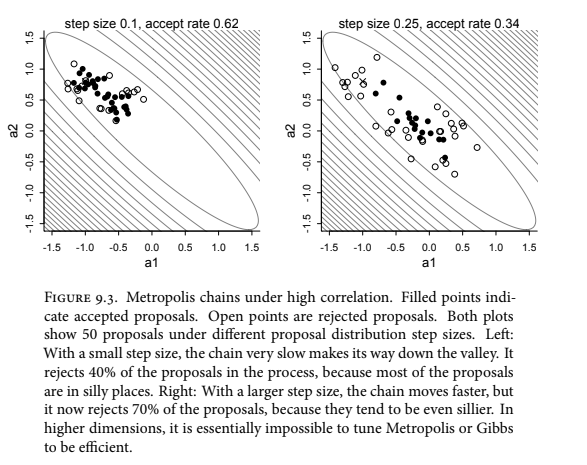
So far, both the Metropolis algorithm and Gibbs sampling seem like remarkably elegant solutions to the problem of sampling from an intractable posterior. And for simple, low-dimensional problems — like Prof. Markov navigating a 5×5 grid with a single unknown — they work beautifully. But as models grow in complexity, both algorithms develop the same fundamental weakness: they get shockingly inefficient, and in high enough dimensions, they effectively stop working altogether. There are two reasons for this.
Figure 9.3. Metropolis chains under high correlation.#

9.2.2.2. Problem 2 — Concentration of Measure#
The step size trap becomes more manageable with careful tuning in low dimensions. But there is a second, more fundamental problem that no amount of tuning can fix: As the number of parameters grows, the geometry of high-dimensional probability distributions becomes deeply counterintuitive in a way that breaks any sampler that explores the posterior one or a few dimensions at a time.
To understand this, let’s start with something familiar. Imagine a Gaussian distribution in two dimensions — a smooth hill, highest at the centre and tapering off symmetrically in all directions. The peak of the hill, the mode, is the single point of highest probability density. But here is the question that matters: If you filled that hill with dirt, where would most of the dirt be? It won’t be at the peak. As you move outward from the peak in any direction, the height drops but the area of the ring at that distance grows. A thin ring far from the peak contains far more total dirt than the tiny patch right at the summit. So the total probability mass (i.e. the dirt) is not concentrated at the mode at all. It lives in a ring some distance away from it where the decrease in height is more than compensated for by the increase in area.
In three dimensions the same logic applies: Not a ring but a spherical shell. And again the bulk of the probability mass lives in that shell rather than at the dense core. This phenomenon is called concentration of measure where most of the probability mass of a distribution lives far from its mode, in a shell whose distance from the mode grows with dimensionality.
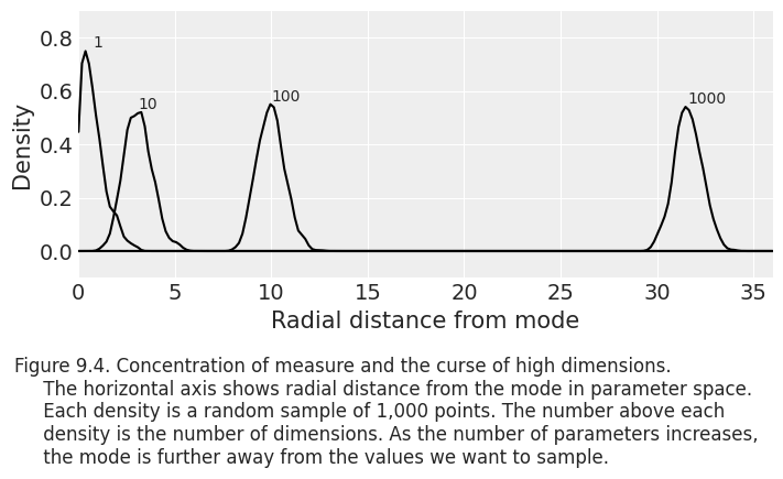
Now consider what happens as we push this into higher and higher dimensions. We’ve run the code in Figure 9.4 where we draws 1,000 random samples from a standard Gaussian in 1, 10, 100, and 1,000 dimensions, and plots how far each sampled point sits from the mode. In one dimension, almost all samples land right next to the mode, exactly what you’d intuitively expect. But in 10 dimensions, no samples land near the mode at all and the distribution of sampled points has already shifted noticeably outward. In 100 dimensions, the typical sample is radial distance 10 away from the mode. In 1,000 dimensions, it’s around distance 32. The sampled points are living in a thin, high-dimensional shell that is geometrically very far from the peak of the distribution and inside that shell, pairs of parameters curve dramatically against one another, creating narrow, winding paths that are extraordinarily difficult to follow.
The practical consequence for Prof. Markov is this. If his model had not 2 unknowns but 200, which is a realistic number for a serious spatial wildfire model with dozens of environmental covariates, random effects, and uncertainty at multiple levels, then the region of parameter space that actually contains meaningful posterior probability is a thin curved shell in 200-dimensional space. Far from the mode. A sampler that takes random steps in one or a few dimensions at a time like Metropolis or Gibbs has almost no chance of staying on that shell. It will either fall off it into low-probability territory and get rejected, or shuffle so slowly along it that it never meaningfully explores the full posterior in any practical amount of time.
This is precisely why the conjugacy requirement of Gibbs, which is already a constraint in low dimensions, becomes completely untenable as models grow. Not every prior-likelihood combination has a clean closed-form conditional posterior and even when conjugate pairs exist, the one-parameter-at-a-time updating strategy is fundamentally ill-suited to the curved, high-dimensional geometry that complex models produce. What we need is an algorithm that doesn’t explore the posterior blindly one dimension at a time but instead uses knowledge of the global shape of the posterior to make informed, efficient proposals that stay on the high-probability shell regardless of how many dimensions it curves through. That algorithm is Hamiltonian Monte Carlo which is the subject of the next section.
Figure 9.4. Concentration of measure and the curse of high dimensions.#
Code 9.4#
def rad_dist(Y):
    return np.sqrt(np.sum(Y**2))


fig, ax = plt.subplots(1, 1, figsize=[7, 3])
xvar = np.linspace(0, 36, 200)

# the book code is wrapped in a loop to reproduce Figure 9.4
for D in [1, 10, 100, 1000]:
    # Constructs a T x D matrix of sampled values
    T = 1000  # int(1e3)
    Y = stats.multivariate_normal(np.zeros(D), np.identity(D)).rvs(T)

    Rd = list(map(rad_dist, Y))

    kde = stats.gaussian_kde(Rd)
    yvar = kde(xvar)
    ax.plot(xvar, yvar, color="k")

    ax.text(np.mean(Rd), np.max(yvar) * 1.02, f"{D}")

ax.set_xlim(0, 36)
ax.set_xlabel("Radial distance from mode")
ax.set_ylim(-0.1, 0.9)
ax.set_ylabel("Density")

#####################
### CODE ADDITION ###
#####################
plt.suptitle(
    x=0.5,
    y=-0.06,
    t="Figure 9.4. Concentration of measure and the curse of high dimensions. \n \
    The horizontal axis shows radial distance from the mode in parameter space. \n \
    Each density is a random sample of 1,000 points. The number above each \n \
    density is the number of dimensions. As the number of parameters increases,  \n \
    the mode is further away from the values we want to sample.",
    ma="left"
  );
Section 9.3 - Hamiltonian Monte Carlo#
It appears to be a quite general principle that, whenever there is a randomized way of doing something, then there is a nonrandomized way that delivers better preformance but requires more thought.
-E. T. Jaynes.
Metropolis and Gibbs sampling are highly random procedures that propose new parameter values and evaluate them to see how good they are compared to the current value. Gibbs sampling takes a step towards using less randomized methods by exploiting knowledge of the target distribution. This pattern seems to fit Jaynes’ observation that when there’s a randomized way of accomplishing some calculation then a less random method comes along with better preformance at the cost of more careful thought required towards the procedure.
Hamiltonian Monte Carlo (HMC), previously also called Hybrid Monte Carlo, pushes Jayne’s principle much further by being able to sample more efficiently to describe the posterior distribution at the cost of being more computationally expensive than either the Metropolis or Gibbs flavour of MCMC. Where HMC really shines is in sampling models that are more complex, even in the range of tens of thousands of parameters, which would break other sampling methods.
9.3.1. Hamilton’s courrier services.#
To illustrate how the Hamilton Monte Carlo algorithm works, we’ll now tell a story of Prof Markov’s nephew, Hamilton, and the small business he runs in his community. Hamilton is a bicycle courier delivering packages across a valley on Vancouver Island. The town he serves sits at the lowest point in the valley beside a river running through it, with mountains, as well as a single road, rising to the north and south of the town. Most of Hamilton’s customers live in town near the valley floor, with the distribution of residents thinning out the farther away he goes. Fewer live partway up the slopes and almost nobody lives near the peaks.
Due to the nature of his work, Hamilton doesn’t plan his routes because he’s simply responding to whatever delivery comes in. Those requests arrive from unpredictable directions — sometimes calling him north of his current location, or sometimes south at the other end of the valley. Also, the amount of effort he puts in to kicking off and initiating the first few pedals to gain momentum varies greatly because like most of us, some mornings Hamilton feels lazier than others! So in summary, the initial direction of his travels and the effort he puts in to pushing off and pedalling are all genuinely left to chance.
Once Hamilton gets going though, chance disappears entirely and the terrain takes over. Gravity governs every subsequent change in his speed. Heading downhill towards town propels him to pick up speed without any effort at all. When heading uphill into the sparser areas of town, he loses speed fighting the climb, and how far he gets depends entirely on how much of that initial push he had left. Not to mention all the slopes and hills within the valley and up the mountains creating the variability in terrain and effort level. A modest effort gets him only partway up the mountain before he stalls while a strong one can carry him clear across the valley floor and partway up slope before he finally runs out of steam.
However, Hamilton doesn’t quit pedalling just because he’s winded. Years on the job have built up his stamina. He only stops for a snack only once he runs out of steam and gravity has nothing left to give, wherever in the valley that happens to leave him.
Prof Markov, watching his nephew’s rounds over the years, noticed something worth proving. He didn’t need to survey a single household to know where was the most densely populated areas. Instead, he could just tally how often Hamilton stopped at each point along the valley. Markov’s reasoning was that naturally, the proportion of time Hamilton spends in each area of the valley must reflect the distribution of his customers’ residences as he’s the only courier in the valley. Therefore the spots where chance and gravity kept bringing Hamilton should turn out to match the town’s population density almost exactly.
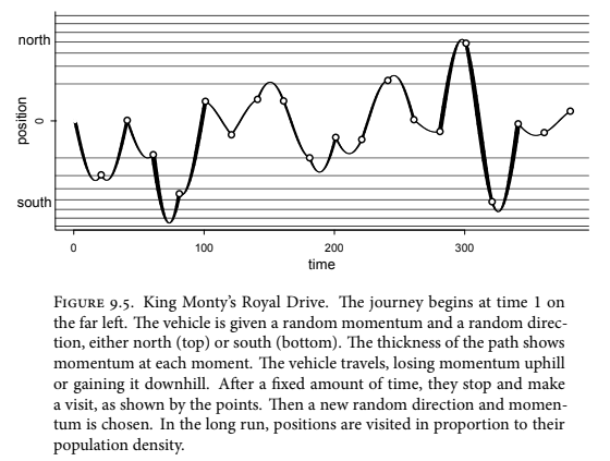
A similar graph on Figure 9.5 can just as well simulate Hamilton’s typical movement patterns and effort level throughout his working day. The horizontal axis is time while the vertical axis is his position in the valley, north or south of town. The thickness of the path at any moment represents his speed: Thick where he’s flying downhill with real momentum and thin where he’s straining himself going uphill and fighting against the urge to stall. The open circles mark the end of each leg, the delivery point where one trip ends and the next begins. Because each leg strikes off in a fresh random direction with a fresh burst of effort, knowing which way Hamilton just came from tells you almost nothing about which way he’ll head next since consecutive legs are essentially uncorrelated. Compare that to another hypothetical courier who only ever wanders to a neighboring address one block at a time: The autocorrelation, which is a measure of how similar a sequence of values is to itself at different time lags, in their route is inherently high because knowing the location of one of their deliveries tells us something about the next one.
Through observation, Prof Markov inadvertently figured out a way to build a census and population distribution using his newphew’s delivery log which we, as readers, can use as a mental model for understanding how the HMC-flavour of MCMC works.
Figure 9.5. King Monty’s Royal Drive.#

Rethinking: Hamiltonians.#
Funny fact: The Hamilton who gave rise to HMC actually had nothing to do with the development of the algorithm. Sir William Rowan Hamiltion (1805-1865), one of the greatest mathematicians and physicists of his generation, was actually known for reformulating Newton’s Laws of Motions into a new system we now call Hamiltonian Mechanics (or Dynamics). Hamiltonian Monte Carlo was named as such more so by the differential equations from Hamiltonian Mechanics which drive it!
9.3.2. Particles in space.#
As you’ve probably guessed, the story of Prof Markov’s nephew, Hamilton the courier, is analogous to how the actual Hamiltonian Monte Carlo MCMC algorithm works. In our parable which functions as a single-parameter case, Hamiltion himself and his bike represent a one number - the parameter’s current value as it moves along a 1D valley. In an actual statistical model, we could think of Hamilton as one particle whose position needs \(x\)-number of coordinates represented as a collection/vector of parameter values, such as a slope value, a y-intercept, or a standard deviation. Another way to think of the Hamilton particle is that it represents coodinates in a multi-dimensional space such as the point \((\alpha, \beta, \sigma) = (1.2, 0.4, 0.9)\) being in a single position in space.
On the otherhand, the log-posterior is like the bowl-shaped valley where the highest posterior probability is in the lowest point (i.e. the centre) of the valley. To generate a sample, we need give the Hamilton particle a flick by assigning an independent and random “momentum value” to every dimension at once, then simulate exactly one full leg of his journey, letting the valley’s slope decelerate or accelerate him along the way. Wherever the particle ends up when that leg concludes becomes the one sample we record, before a fresh flick launches the next leg from there.
In practice, HMC truly does a physics simulation of the “Hamilton particle” moving along a surface of log-posteriors. When the log-posterior is flat due to the lack of information in the likelihood or because of flat priors, the particle can coast for awhile before being forced to turn around. The opposite happens when the log posterior is steep so the particle isn’t able to go very far.
Similar to Metropolis-Hastings, HMC also uses a rejection criterion. However, it’s quite normal to see acceptance rates of over 95% with HMC because it only makes intelligent proposals by approximating the smooth path or a particle. The high level overview of the rejection criterion for HMC is that its based on the total energy conserved in the system when simulating a particle’s trajectory. HMC’s accept/reject criterion exists specifically to catch cases where numerical error violated that conservation.
In order to generate intuition about why HMC works over other approaches and when it doesn’t, let’s play with the example of a dataset with 100 \(x\) and \(y\) values each sampled from a \(\text{Normal}(0, 1)\) distribution using the model:
\( x_i \sim \text{Normal}(\mu_x, 1)\)
\( y_i \sim \text{Normal}(\mu_y, 1)\)
\( \mu_x \sim \text{Normal}(0.05, 1)\)
\( \mu_y \sim \text{Normal}(0.05, 1)\)
To initialize a sample using the HMC mechanism, we’ll need two functions and two settings.
The first function computes the log-probability of the data and parameters so that the algorithm knows what the “elevation” is of a given set of parameter values. For our model, the function for log-probability is the following:
\[ \sum_i \log p(y_i|\mu_y, 1) + \sum_i \log p(x_i|\mu_x, 1) + \log p(\mu_y|0, 0.5) + \log p(\mu_x | 0, 0.5) \]Where:
\( p(x | a, b) \) is the Gaussian density of \(x\) at mean of \(a\) and standard deviation of \(b\). So in essence, every line in our model needs to be added to one another.
The second function HMC needs is a gradient which is a separate slope measurement for each individual parameter in the model. With our model, since we have two parameters, \(\mu_x\) and \(\mu_y\), our gradient then has two components: One is a derivative value telling us how steep the log-posterior rises or falls as \(\mu_x\) changes (holding \(\mu_y\) constant), and the other telling us the same thing for \(\mu_y\) holding \(\mu_x\) constant. If there’s 10 parameters in our model, we’ll get exactly 10 derivative values. Each one of those derivatives asks a very specific quesiton: “If I nudge this one parameter slightly, holding every other parameter constant, does the log-posterior increase or decrease, and how quickly?
Conversely, the two setting that HMC needs is the choice of the number of leapfrog steps and a choice of the step size for each.
The length of each line in Figure 9.5 is divided by the number of leapfrog steps and the step size. The greater the value of the leapfrog steps you chose, the longer the path, and fewer leapfrog steps result in shorter paths.
On the otherhand, the step size determines how granular the simulation is since it determines the size of each leapfrog step. Small step sizes mean sharper turns for the particle. And with larger step sizes comes larger leapfrog steps which could result in situations where the particle shoots past its target point and needs to turn around.
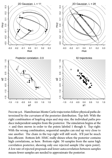
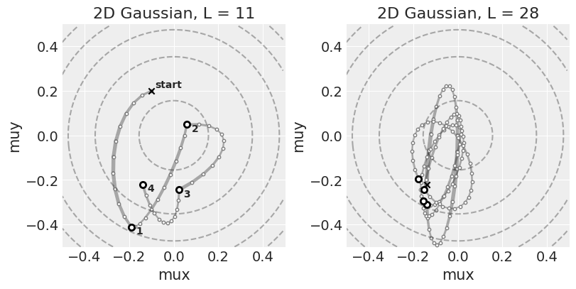
Let’s now bring these concepts to life with Figure 9.6. The code to reproduce this figure is in the Overthinking box below. The top-left panel uses \(L = 11\) leapfrog steps, each with a step size of \(\epsilon = 0.03\). Before looking at the results, it’s worth understanding what these two numbers actually control since they operate on very different scales. The step size \(\epsilon\) is the distance the simulation moves in a single leapfrog step and 0.03 is tiny relative to the plot’s own scale since both axes only span from −0.3 to 0.3. \(L\) is simply the count of how many of these small steps make up one full trajectory before we stop and record a sample. So a trajectory with \(L = 11\) and \(\epsilon = 0.03\) traces a path roughly \(11 × 0.03 ≈ 0.33\) units long, which is a substantial fraction of the whole plot built from 11 tiny, evenly-spaced increments rather than one large leap.
The contours in the top-left panel show the log-posterior which forms a symmetric bowl in this example. Only 4 samples are shown, and the chain begins at the \(×\). The first trajectory gets flicked to the right, rolls downhill, and stops there, thus completing our recording of the first sample at the point labeled 1. The width of the path at any point reflects the total momentum (kinetic energy) at that instant and each individual leapfrog step along the way is marked by a white dot. This same process then repeats three more times, each with a fresh random direction and momentum, producing samples 2, 3, and 4. With this combination of \(L\) and \(\epsilon\), you could take 100 samples from this simulation and get an excellent approximation of the posterior with very low autocorrelation between them.
However, that low autocorrelation is not guaranteed as it depends entirely on getting \(L\) and \(\epsilon\) right. The top-right panel runs the identical code, but with \(L\) increased to 28 while \(\epsilon\) stays the same. Since \(\epsilon\) is unchanged, each individual step is still just as small. But with more than double the steps, the trajectory now travels roughly \(28 × 0.03 ≈ 0.84\) units, more than twice as far as before. That extra distance is precisely the problem since the path now travels so far that it curves back around and lands close to where it started. Rather than producing independent samples the way the top-left panel did, the top-right panel now generates correlated samples that bring us the same failure modes that plagued ordinary Metropolis chains.
This problem is called the U-turn problem where the simulated trajectory travels far enough to loop back on itself and return to the neighbourhood it started from. It looks especially dramatic here because this particular posterior is a perfectly symmetric 2-dimensional Gaussian bowl so the parabolic paths curve back on themselves in a very clean, visible way. Most real posteriors won’t be quite this symmetric, but the same underlying risk remains: A poorly chosen combination of \(L\) and \(\epsilon\) can still send a trajectory looping back near its own starting point. This is the central tradeoff of HMC: The efficiency gains over Metropolis and Gibbs come at the cost of having to tune the number of leapfrog steps and the step size for each new model you build.
Fancy HMC samplers like PyMC use the No-U-Turn Sampler (NUTS), which automatically detects when a trajectory starts to double back on itself and stops the simulation right before that happens, rather than relying on a fixed, manually-tuned number of leapfrog steps (\(L\)). It also automatically tunes the step size (\(\epsilon\)) during a warm-up phase to hit a target acceptance rate by guessing the shape of the posterior when the path is turning around. That way, you never have to hand-pick either setting value the way we had to in Figure 9.6. And to clarify, a warm-up phase is when a sampler tries to figure out which step size explores the posterior efficiently to tune the simulation.
Figure 9.6. Hamiltonian Monte Carlo trajectories by the curvature of the posterior distribution.#

Overthinking: Hamiltonian Monte Carlo in the raw.#
The Hamiltonian Monte Carlo MCMC algorithm needs \(5\) things in order to get going:
The function
calc_U()that calculates the negative log-probability of the data at the current position (i.e. the parameter values);The
calc_U_gradientfunction that returns the gradient of the negative log-probability as its current position (also called the loss function in ML circles);The step size (\(\epsilon\));
The number of leapfrog steps (\(L\));
And a starting position (
current_q).
Keep in mind that the particle’s position is a vector of parameters that represent a coordinate in an \(x\)-dimensional space so the gradient also needs to return a vector of \(x\)-length.
print("Generating our test data... \n\n")

np.random.seed(42)

# test data
real = stats.multivariate_normal([0, 0], np.identity(2))
x, y = real.rvs(50).T

print(f"x (length: {len(x)}): {x}, \n\n \
y (length: {len(y)}): {y}")
Generating our test data...


x (length: 50): [ 0.49671415  0.64768854 -0.23415337  1.57921282 -0.46947439 -0.46341769
  0.24196227 -1.72491783 -1.01283112 -0.90802408  1.46564877  0.0675282
 -0.54438272 -1.15099358 -0.60063869 -0.60170661 -0.01349722  0.82254491
  0.2088636  -1.32818605  0.73846658 -0.11564828 -1.47852199 -0.46063877
  0.34361829  0.32408397 -0.676922    1.03099952 -0.83921752  0.33126343
 -0.47917424 -1.10633497  0.81252582 -0.07201012  0.36163603  0.36139561
 -0.03582604 -2.6197451   0.08704707  0.09176078 -0.21967189  1.47789404
 -0.8084936   0.91540212 -0.5297602   0.09707755 -0.70205309 -0.39210815
  0.29612028  0.00511346],

 y (length: 50): [-0.1382643   1.52302986 -0.23413696  0.76743473  0.54256004 -0.46572975
 -1.91328024 -0.56228753  0.31424733 -1.4123037  -0.2257763  -1.42474819
  0.11092259  0.37569802 -0.29169375  1.85227818 -1.05771093 -1.22084365
 -1.95967012  0.19686124  0.17136828 -0.3011037  -0.71984421  1.05712223
 -1.76304016 -0.38508228  0.61167629  0.93128012 -0.30921238  0.97554513
 -0.18565898 -1.19620662  1.35624003  1.0035329  -0.64511975  1.53803657
  1.56464366  0.8219025  -0.29900735 -1.98756891  0.35711257 -0.51827022
 -0.50175704  0.32875111  0.51326743  0.96864499 -0.32766215 -1.46351495
  0.26105527 -0.23458713]
Code 9.5#
The following calc_U() function represents the log posterior, similar to what we already built in Section 9.3.2:
Here’s our original model again for reference:
\( x_i \sim \text{Normal}(\mu_x, 1)\)
\( y_i \sim \text{Normal}(\mu_y, 1)\)
\( \mu_x \sim \text{Normal}(0.05, 1)\)
\( \mu_y \sim \text{Normal}(0.05, 1)\)
# Q["q"] = np.array([-0.1, 0.2])

def calc_U(x, y, q, a=0, b=1, k=0, d=1):
    mu_y, mu_x = q

    U = (
        np.sum(stats.norm.logpdf(y, loc=mu_y, scale=1))
        + np.sum(stats.norm.logpdf(x, loc=mu_x, scale=1))
        + stats.norm.logpdf(mu_y, loc=a, scale=b)
        + stats.norm.logpdf(mu_x, loc=k, scale=d)
    )

    return -U
Code 9.6#
Now our gradient function calc_U_gradient() requires two partial derivatives but luckily for us, Gaussian derivatives are pretty clean. Think of a derivative as answering the question: “If I nudge this input slightly, how much does the output change?” It’s a measure of sensitivity. For a Gaussian distribution with mean \(a\) and standard deviation \(b\), the sensitivity of its log-probability to changes in the mean \(a\) turns out to have a clean, intuitive form:
In plain terms: The further your observed value \(y\) is from the mean \(a\), the bigger this quantity become. Its sign tells you which direction would make \(y\) more likely under the distribution. Divide that gap by \(b^2\) (the variance) and you get exactly how sensitive the log-probability is to \(a\).
Because a derivative of a sum is just the sum of the individual derivatives (nothing gets tangled together), we can compute the gradient for \(\mu_x\) by simply adding up the sensitivity contributed by each term in our model, one piece at a time:
Here, each data point \(x_i\) contributes a push toward making \(\mu_x\) closer to it (that’s the sum over \(i\)), while the prior belief that \(\mu_x\) should be near 0 contributes its own gentle pull in the opposite direction. Adding these together gives the total “slope” telling us which way to adjust \(\mu_x\) to make the whole model fit better.
Another cleaner way to express the gradient function of the negative log-probability (i.e. loss function) is through the following equation:
\( \frac{\partial U}{\partial \mu_y} = \sum_i (y_i - \mu_y) + \frac{a - \mu_y}{b^2} \)
\(\frac{\partial U}{\partial \mu_x} = \sum_i (x_i - \mu_x) + \frac{k - \mu_x}{b^2}\)
\( \nabla U(\mu_y, \mu_x) = -\left(\frac{\partial U}{\partial \mu_y}, \ \frac{\partial U}{\partial \mu_x}\right) \)
# gradient function
# need vector of partial derivatives of U with respect to vector q
def calc_U_gradient(x, y, q, a=0, b=1, k=0, d=1):
    mu_y, mu_x = q

    G1 = np.sum(y - mu_y) + (a - mu_y) / b**2  # dU/dmuy
    G2 = np.sum(x - mu_x) + (k - mu_x) / d**2  # dU/dmux

    return np.array([-G1, -G2])
Code 9.8 - 9.10#
9.7 uses the function defined here, so is below
The function of HMC2() is based on Radford Neal’s example scripts from his book, Handbook of Markov Chain Monte Carlo. The accept/reject decision for the state of the trajectory follows Hamiltonian dynamics where the total energy of the system must stay constant. So if the energy at the start of the trajectory differs substantially from the energy at the end, this is what’s known as divergent transition which is a signal that something has gone wrong with this chain.
def HMC2(U, grad_U, epsilon, L, current_q, x, y):
    q = current_q
    p = np.random.normal(loc=0, scale=1, size=len(q))  # random flick - p is momentum
    current_p = p

    # Make a half step for momentum at the beginning
    p -= epsilon * grad_U(x, y, q) / 2

    # initialize bookkeeping - saves trajectory
    qtraj = np.full((L + 1, len(q)), np.nan)
    ptraj = qtraj.copy()
    qtraj[0, :] = current_q
    ptraj[0, :] = p

    # Code 9.9 starts here
    # Alternate full steps for position and momentum
    for i in range(L):
        q += epsilon * p  # Full step for the position
        qtraj[i + 1, :] = q

        # Make a full step for the momentum, except at the end of trajectory
        if i != L - 1:
            p -= epsilon * grad_U(x, y, q)
            ptraj[i + 1, :] = p

    # Make a half step for momentum at the end
    p -= epsilon * grad_U(x, y, q) / 2
    ptraj[L, :] = p

    # Negate momentum at end of trajectory to make the proposal symmetric
    p *= -1

    # Evaluate potential and kinetic energies sat start and end of trajectory
    current_U = U(x, y, current_q)
    current_K = np.sum(current_p**2) / 2
    proposed_U = U(x, y, q)
    proposed_K = np.sum(p**2) / 2

    # Accept or reject the state at end of trajectory, returning either
    # the position at the end of the trajectory or the initial position
    accept = False

    if np.random.uniform() < np.exp(current_U - proposed_U + current_K - proposed_K):
        new_q = q  # accept
        accept = True
    else:
        new_q = current_q  # reject

    return dict(q=new_q, traj=qtraj, ptraj=ptraj, accept=accept)
Code 9.7#
This code expands upon 9.7 to produce both panels in the top row of Figure 9.6
Q = {}
Q["q"] = np.array([-0.1, 0.2])
pr = 0.5
step = 0.03
# L = 11  # 0.03 / 28 for U-turns -- 11 for working example
n_samples = 4

_, axs = plt.subplots(1, 2, figsize=[8, 6], constrained_layout=True)

for L, ax in zip([11, 28], axs):
    ax.scatter(*Q["q"], color="k", marker="x", zorder=3)
    if L == 11:
        ax.text(*Q["q"] + 0.015, "start", weight="bold")
    for i in range(n_samples):
        Q = HMC2(U=calc_U, grad_U=calc_U_gradient, epsilon=step, L=L, current_q=Q["q"], x=x, y=y)
        ax.scatter(*Q["q"], color="w", marker="o", edgecolor="k", lw=2, zorder=3)
        if n_samples < 10:
            for j in range(L):
                K0 = np.sum(Q["ptraj"][j, :] ** 2) / 2  # kinetic energy
                ax.plot(
                    Q["traj"][j : j + 2, 0],
                    Q["traj"][j : j + 2, 1],
                    color="k",
                    lw=1 + 1 * K0,
                    alpha=0.3,
                    zorder=1,
                )
            ax.scatter(*Q["traj"].T, facecolor="w", edgecolor="gray", lw=1, zorder=2, s=10)
            if L == 11:
                ax.text(*Q["q"] + [0.02, -0.03], f"{i + 1}", weight="bold")

    ax.set_title(f"2D Gaussian, L = {L}")
    ax.set_xlabel("mux")
    ax.set_ylabel("muy")

    # draw background contours based on real probability defined above
    ax.set_xlim(-pr, pr)
    ax.set_ylim(-pr, pr)
    xs, ys = np.mgrid[-pr:pr:0.01, -pr:pr:0.01]
    p = real.logpdf(np.vstack([xs.flat, ys.flat]).T).reshape(xs.shape)
    ax.contour(xs, ys, p, 4, colors=[(0, 0, 0, 0.3)])
    ax.set_aspect(1);
result = ",  ".join(f"{key} (n = {len(values)})" for key, values in Q.items() if key != 'accept')

print(f"Printing the results of our starting position... \n\n {result}")
Printing the results of our starting position...

 q (n = 2),  traj (n = 29),  ptraj (n = 29)
# Figure 9.6 (bottom row) with correlated data

np.random.seed()

# test data
realc = stats.multivariate_normal([0, 0], [[1, -0.9], [-0.9, 1]])  # generate correlated data
x, y = real.rvs(50).T

Q = {}
pr = 0.6
step = 0.03
L = 21  # 28 for U-turns -- 11 for working example

_, axs = plt.subplots(1, 2, figsize=[8, 4], constrained_layout=True)

for n_samples, ax in zip([4, 50], axs):
    Q["q"] = np.array([-0.3, 0.3])

    ax.scatter(*Q["q"], color="k", marker="x", zorder=3)
    if n_samples == 4:
        ax.text(*Q["q"] + 0.015, "start", weight="bold")
    for i in range(n_samples):
        Q = HMC2(calc_U, calc_U_gradient, step, L, Q["q"], x, y)
        ax.scatter(*Q["q"], color="w", marker="o", edgecolor="k", lw=2, zorder=3)
        if n_samples < 10:
            for j in range(L):
                K0 = np.sum(Q["ptraj"][j, :] ** 2) / 2  # kinetic energy
                ax.plot(
                    Q["traj"][j : j + 2, 0],
                    Q["traj"][j : j + 2, 1],
                    color="k",
                    lw=1 + 1 * K0,
                    alpha=0.3,
                    zorder=1,
                )
            if Q["accept"]:
                c = "w"
            else:
                c = "k"
            ax.scatter(*Q["traj"].T, facecolor=c, edgecolor="gray", lw=1, zorder=2, s=10)
            if n_samples == 4:
                ax.text(*Q["q"] + [0.02, -0.03], f"{i + 1}", weight="bold")

    ax.set_title(f"Correlation -0.9")
    ax.set_xlabel("mux")
    ax.set_ylabel("muy")

    # draw background contours based on real probability defined above
    ax.set_xlim(-pr, pr)
    ax.set_ylim(-pr, pr)
    xs, ys = np.mgrid[-pr:pr:0.01, -pr:pr:0.01]
    p = realc.logpdf(np.vstack([xs.flat, ys.flat]).T).reshape(xs.shape)
    ax.contour(xs, ys, p, 5, colors=[(0, 0, 0, 0.3)])
    ax.set_aspect(1);
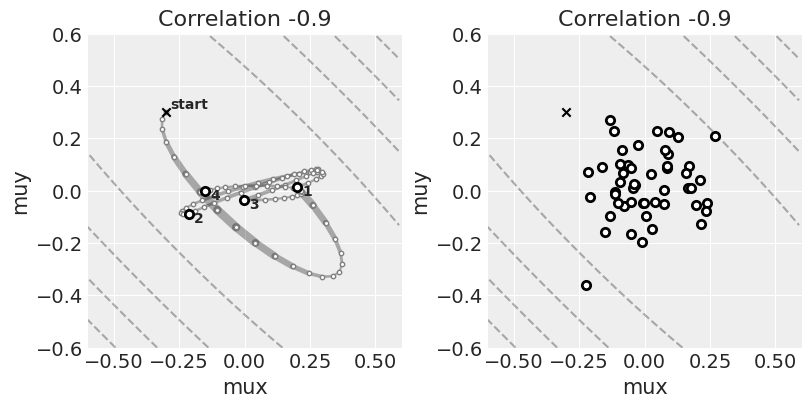
The correlated case doens’t work as well as the uncorrelated case, compared to the book. We’re not reproducing the sinusoid trajectories that are shown in the book, so it’s possible that there was some underlying change in the likelihood functions? The book doesn’t provide code or parameters used to recreate these plots, so we’re guessing blind here.
9.3.3. Limitations.#
There’s two limitations we need to be aware of with HMC. The first is that HMC requires continuous variables to sample, not discrete/categorical ones. This requirement also means that HMC can’t handle missing data directly so we’ll need to ensure that our data/likelihoods are clean before feeding them to a Bayesian model using an MCMC sampler.
The other issue is that HMC is not a magic bullet and may struggle to sample from posterior distributions that are inherently difficult to sample from, despite your algorithm of choice. As we mentioned earlier, the problem of divergent transition is often the main culprit behind issues that HMC can struggle with.
Section 9.4 - Easy HMC: ulam#
Here I won’t focus too much on the summary explanations of this section as we’re using PyMC in this notebook. I’ll only highlight some key points of this section…
Code 9.11#
rugged_csv = "https://raw.githubusercontent.com/vanislekahuna/Statistical-Rethinking-PyMC/refs/heads/main/Data/rugged.csv"
d = pd.read_csv(rugged_csv, delimiter=";")

d["log_gdp"] = np.log(d["rgdppc_2000"])

dd = d.dropna(subset=["log_gdp"])
dd["log_gdp_std"] = dd["log_gdp"] / dd["log_gdp"].mean()
dd["rugged_std"] = dd["rugged"] / dd["rugged"].max()

d.head()
| isocode | isonum | country | rugged | rugged_popw | rugged_slope | rugged_lsd | rugged_pc | land_area | lat | ... | africa_region_e | africa_region_c | slave_exports | dist_slavemkt_atlantic | dist_slavemkt_indian | dist_slavemkt_saharan | dist_slavemkt_redsea | pop_1400 | european_descent | log_gdp | |
|---|---|---|---|---|---|---|---|---|---|---|---|---|---|---|---|---|---|---|---|---|---|
| 0 | ABW | 533 | Aruba | 0.462 | 0.380 | 1.226 | 0.144 | 0.000 | 18.0 | 12.508 | ... | 0 | 0 | 0.0 | NaN | NaN | NaN | NaN | 614.0 | NaN | NaN |
| 1 | AFG | 4 | Afghanistan | 2.518 | 1.469 | 7.414 | 0.720 | 39.004 | 65209.0 | 33.833 | ... | 0 | 0 | 0.0 | NaN | NaN | NaN | NaN | 1870829.0 | 0.0 | NaN |
| 2 | AGO | 24 | Angola | 0.858 | 0.714 | 2.274 | 0.228 | 4.906 | 124670.0 | -12.299 | ... | 0 | 1 | 3610000.0 | 5.669 | 6.981 | 4.926 | 3.872 | 1223208.0 | 2.0 | 7.492609 |
| 3 | AIA | 660 | Anguilla | 0.013 | 0.010 | 0.026 | 0.006 | 0.000 | 9.0 | 18.231 | ... | 0 | 0 | 0.0 | NaN | NaN | NaN | NaN | NaN | NaN | NaN |
| 4 | ALB | 8 | Albania | 3.427 | 1.597 | 10.451 | 1.006 | 62.133 | 2740.0 | 41.143 | ... | 0 | 0 | 0.0 | NaN | NaN | NaN | NaN | 200000.0 | 100.0 | 8.216929 |
5 rows × 52 columns
Code 9.12-9.18#
By using PyMC we are already doing everything in these code blocks (No-U-turn sampling, parallell processing).
To translate the results of summary to rethinking’s precis:
n_eff = ess_bulk: A crude estimate of the number of independent samples we got. The difference with the ArViz version is that the effective sample size is based on rank-normalized draws, which is what’s actually being estimated when we care about the reliability of the mean or median.Rhat4 = r_hat: A complicated estimate of the convergence of the Markov chains to the target distribution. It should approach1.00or more when all is well.
These two columns are a MCMC diagnostic criteria to tell us how well our sampling worked.
cid = pd.Categorical(dd["cont_africa"])

with pm.Model() as m_8_3:
    a = pm.Normal("a", 1, 0.2, shape=cid.categories.size)
    b = pm.Normal("b", 0, 0.3, shape=cid.categories.size)

    mu = a[np.array(cid)] + b[np.array(cid)] * (dd["rugged_std"].values - 0.215)
    sigma = pm.Exponential("sigma", 1)

    log_gdp_std = pm.Normal("log_gdp_std", mu, sigma, observed=dd["log_gdp_std"].values)

    m_8_3_trace = pm.sample()

az.summary(m_8_3_trace, kind="all", round_to=2)
| mean | sd | hdi_5.5% | hdi_94.5% | mcse_mean | mcse_sd | ess_bulk | ess_tail | r_hat | |
|---|---|---|---|---|---|---|---|---|---|
| a[0] | 1.05 | 0.01 | 1.04 | 1.07 | 0.0 | 0.0 | 2611.07 | 1425.03 | 1.0 |
| a[1] | 0.88 | 0.02 | 0.86 | 0.91 | 0.0 | 0.0 | 2663.81 | 1803.78 | 1.0 |
| b[0] | -0.14 | 0.06 | -0.23 | -0.05 | 0.0 | 0.0 | 2999.30 | 1697.83 | 1.0 |
| b[1] | 0.13 | 0.07 | 0.02 | 0.25 | 0.0 | 0.0 | 2802.50 | 1722.91 | 1.0 |
| sigma | 0.11 | 0.01 | 0.10 | 0.12 | 0.0 | 0.0 | 3113.83 | 1800.81 | 1.0 |
Figure 9.7. Pairs plot of the samples produced by arviz.#
Code 9.19#
axes_97 = az.plot_pair(m_8_3_trace, figsize=[11, 11], marginals=True)


#####################
### CODE ADDITION ###
#####################
fig = axes_97.ravel()[0].get_figure()
fig.suptitle(
  x=0.5,
  y=-0.06,
  t=r"Figure 9.7. Pair plot of the samples produced by $\mathtt{arviz}$. The diagonal shows a density estimate for each parameter.",
)

plt.tight_layout();
/tmp/ipykernel_825/985483963.py:14: UserWarning: The figure layout has changed to tight
  plt.tight_layout();
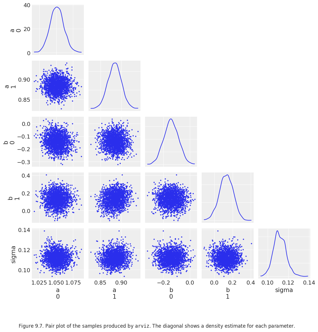
Figure 9.8. Trace plot of the Markov chain from the ruggedness model, m_8_3.#
Code 9.20#
We know a when a Markov chain is a healthy one by looking for 3 characteristics from these trace plots:
Stationarity which refers to the path of each chain staying within the same high-probability portion of the posterior distribution. In other words, not jumping around wildly and staying close to a stable central tendency;
Good mixing means that the chain rapidly explores the full region. It doesn’t slowly wander around but instead rapidly zig-zags around like we saw with the left-side graphs of Figure 9.6;
Convergence means the multiple independent chains stick around the same region of high probability.
axes_98 = az.plot_trace(m_8_3_trace, figsize=[8, 8])

#####################
### CODE ADDITION ###
#####################
fig = axes_98.ravel()[0].get_figure()
fig.suptitle(
  x=0.35,
  y=-0.06,
  t=r"Figure 9.8. Trace plot of the Markov chain from the ruggedness model, $\mathtt{m\_8\_3}$. \n \
  This is a clean, healthy Markov chain, both stationary and well-mixing.",
)

plt.tight_layout();
/tmp/ipykernel_825/1324483294.py:14: UserWarning: The figure layout has changed to tight
  plt.tight_layout();
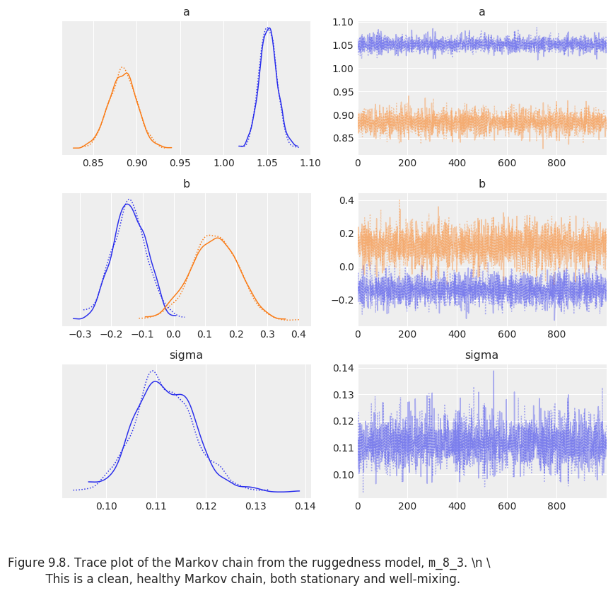
Figure 9.9. Stacked histograms of ranked samples, a trace rank plot, or trank plot, for m_8_3.#
Code 9.21#
In a trace rank plot (trank plot), what it’s doing here is visualizing the chains by plotting the distribution of ranked samples on a histogram. The lowest rank gets 1 and the largest value gets the maximum rank (i.e. the number of samples across the chains which in this case is 2,000). The reasoning behind this is if the chains are exploring the sample space efficiently than the values for each rank should be largely similar and relatively uniform.
axes_99 = az.plot_trace(m_8_3_trace, figsize=[8, 8], kind="rank_bars")


#####################
### CODE ADDITION ###
#####################
fig = axes_99.ravel()[0].get_figure()
fig.suptitle(
  x=0.35,
  y=-0.06,
  t=r"Figure 9.9. Stacked histograms of ranked samples, a trank plot, for $\mathtt{m\_8\_3}$. \n \
  In a healthy chain, these histograms should be reasonable uniform, with no  \n \
  chain consistently running above or below the others.",
)

plt.tight_layout();
/tmp/ipykernel_825/4278345689.py:16: UserWarning: The figure layout has changed to tight
  plt.tight_layout();
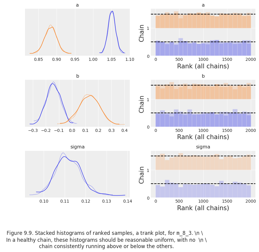
Section 9.5 - Care and feeding of your Markov chain#
It’s natural to feel uneasy about knowing exactly what’s happening under the hood of MCMC and that’s ok. Science requires a division of labour so if everyone had to write their own Markov Chain Monte Carlo sampler from scratch, then a lot less research would be done as a whole which wouldn’t be a good outcome. The important thing to build here is to gain a good intuition of how MCMC works and when to know when it’s complaining. Luckily for us, the best feature of MCMC is actually the fact that it’s easy to visualize and that it complains loudly when things aren’t right so we’ll need to learn some guidelines for how to run these chains.
9.5.1 How many sampled do you need?#
The number of effective samples you need for accurate inference depends largely on the question you’re trying to answer. For example if all you’re looking for is an estimate of the posterior mean, you don’t need more than a couple hundred samples to accomplish this. Another example is that for a typical regression application, it’s possible to achieve a good estimate of the posterior with as little as 200 effective samples. In PyMC, you can use the draws parameter within the .sample() model function to set the number of samples that MCMC can draw from within the posterior. If you don’t specify a number for this parameter, the default argument here is 1,000.
Markov chains has the property of being autocorrelated which means that their sequential samples are not entirely independent. However, PyMC’s defaults are engineered so that for a well-behaved, correctly-specified model, you don’t need to think hard producing autocorrelated samples most of the time. PyMC accomplishes this through it’s use of the NUTS sampler which is engineered to overcome autocorrelation directly at the sampling level. NUTS uses the posterior’s gradient to propose large, informed jumps rather than small blind steps, then automatically tunes step size via dual averaging, and lastly it stops each trajectory the moment it detects a U-turn so that nearly every draw lands far from the last one instead of clustering nearby. Therefore, PyMC’s modest default of 1,000 draws across 4 chains is usually enough for reliable inference athough it’s still worth checking metrics like ESS and R-hat to verify this rather than assuming this holds for every model.
9.5.2. How many chains do you need?#
As we’ve already mentioned, the default number of chains in PyMC is 4 as it’s based on the number of cores or CPUs you have in your system. One chain typically runs on a single processor so they can run simultaneously. If your system has less than 4 cores, the default lowest number of chains that run in a single session is then 2.
For debugging a model, the best practice here is only to use a single chain in this situation for the following reasons:
To check whether a model runs at all;
To check whether the log-probability is well-defined at the initial values;
Or to check whether divergences or errors are structural (bad priors, unidentifiable parameters, shape mismatches) rather than sampling noise.
A single short chain gets us fast, cheap feedback on these issues. PyMC also provides a brief introduction on how to debug their models as well if we need more resources on this topic.
Rethinking: Convergence diagnostics.#
As mentioned earlier, the default diagnostic outputs from PyMC are ess_bulk, which is the effective number of samples per parameter, and r_hat, which is the Gelman-Rubin convergence diagnostic. When ess_bulk is lower than the actual number of iterations in our chain, it means the chains are inefficient but possibly still ok.
When r_hat is above 1.00, it usually indicates that the chains have not yet converged so we shouldn’t trust the samples. Drawing more iterations should fix this problem but there’s also the possibility that the chains never converge.
While helpful, it’s also important not to rely on these diagnostic heuristics too much. An example of this would be that there are cases where r_hat may reach 1.00 with an invalid chain. Therefore, the way to think about these diagnostics is to view them as a signal of danger but never as a signal for safety.
9.5.3. Taming a wild chain.#
A common problem with most models are that they may have broad, flat regions of posterior density which is typical when the model uses flat priors. In such cases, the result then becomes a wild, wandering Markov chain that erratically samples extremely positive, and negative, parameter values.
Code 9.22#
Below is an example of a model (m_9_2) that tries to estimate the mean and standard deviation of a Gaussian dataset/likelihood with only two observations, \(-1\) and \(1\), and extremely flat priors: 😆
y = np.array([-1, 1])

with pm.Model() as m_9_2:
    alpha = pm.Normal("alpha", 0, 1000)

    mu = alpha
    sigma = pm.Exponential("sigma", 0.0001)

    yp = pm.Normal("y", mu, sigma, observed=y)

    m_9_2_trace = pm.sample(chains=3)
ERROR:pymc.stats.convergence:There were 465 divergences after tuning. Increase `target_accept` or reparameterize.
ERROR:pymc.stats.convergence:The effective sample size per chain is smaller than 100 for some parameters.  A higher number is needed for reliable rhat and ess computation. See https://arxiv.org/abs/1903.08008 for details
Code 9.23#
Based on the arviz.summary() function, we can see that the mean for the alpha mean parameter is quite distant from the prior we set at 0 with an implausibly wild interval. Also based on the 2,000 samples we drew from our likelihood dataset of 2 values, but the effective sample size from both parameters are about 824 and 43 which isn’t good.
Also, PyMC returned some warnings that mimic what we covered in our Rethinking section about conergence diagnostics about chain divergence when r_hat exeeds 1.00, indicating that the chains havne’t diverged:
ERROR:pymc.stats.convergence:There were 361 divergences after tuning. Increase `target_accept` or reparameterize.
Or the possible issue with ess_bulk indicating that our effective sample size is lower than the number of iterations, thus indicating that our chains were inefficient:
ERROR:pymc.stats.convergence:The effective sample size per chain is smaller than 100 for some parameters. A higher number is needed for reliable rhat and ess computation. See https://arxiv.org/abs/1903.08008 for details
az.summary(m_9_2_trace, round_to=2)
| mean | sd | hdi_5.5% | hdi_94.5% | mcse_mean | mcse_sd | ess_bulk | ess_tail | r_hat | |
|---|---|---|---|---|---|---|---|---|---|
| alpha | -2.97 | 357.21 | -500.22 | 450.80 | 15.24 | 33.87 | 726.55 | 461.45 | 1.01 |
| sigma | 661.20 | 1535.14 | 18.90 | 1414.33 | 77.93 | 178.83 | 73.89 | 29.80 | 1.03 |
The trace plot in Figure 9.10 shows a model that has failed to converge in a fairly severe way. On the left, the density plots for both alpha and sigma are extremely wide and spread across implausible ranges. alpha stretches from roughly −2500 to 2500, and sigma extends out past 25,000, both of which are wildly larger than any reasonable posterior for a typical regression parameter. This tells us the sampler is exploring parameter space far beyond where the actual probability mass should be concentrated.
On the right, the trace plots (i.e. the “caterpillar” lines showing each chain’s position over iterations) confirm the problem directly. Instead of the tight, fuzzy, overlapping band we’d expect from healthy chains (i.e. the kind that looks like a dense, stationary “hairy caterpillar” oscillating narrowly around a fixed value) these chains show sudden, erratic spikes shooting up to extreme values like 2,000+ for alpha or 20,000+ for sigma at scattered points throughout sampling. This is the signature of a chain occasionally wandering into a region of very low posterior density and getting temporarily stuck or making a wild excursion before snapping back.
# Figure 9.10 (top)
# az.plot_trace(m_9_2_trace, figsize=[8, 3])
The reason we’re seeing our Hamilton particle behave erratically is because of how few data we have and the model’s flat priors. To tame a chain like this, we need to use weakly informative priors so that we can tell the model that every possible value of the parameter is equally plausible. If we give the model an extremely flat prior with implausible values at extreme ends of the distribution, such as saying there 1000 values at either direction when our two data points only went as far as 1, the sampling space would overwhelm the chain!
If we used just even a slightly less extreme, yet weakly informative, prior in this situation, we’ll find that the model’s preformance will improve drastically:
\( y_i \sim \text{Normal}(\mu, \sigma)\)
\( \mu = \alpha \)
\( \alpha \sim \text{Normal}(1, 10)\)
\( \sigma \sim \text{Exponential}(1)\)
Code 9.24#
Model m_9_3 produces the results we see at the bottom half of Figure 9.10 where we can see healthy trace plots for both parameters. Both chains are stationary around the same values and the mixing is good. No wild detours into the thousands and those divergent transitions have gone.
with pm.Model() as m_9_3:
    alpha = pm.Normal("alpha", 1, 10)
    mu = alpha
    sigma = pm.Exponential("sigma", 1)
    yp = pm.Normal("y", mu, sigma, observed=y)
    m_9_3_trace = pm.sample(chains=3)

az.summary(m_9_3_trace, round_to=2)
ERROR:pymc.stats.convergence:There were 6 divergences after tuning. Increase `target_accept` or reparameterize.
| mean | sd | hdi_5.5% | hdi_94.5% | mcse_mean | mcse_sd | ess_bulk | ess_tail | r_hat | |
|---|---|---|---|---|---|---|---|---|---|
| alpha | 0.05 | 1.18 | -1.87 | 1.81 | 0.04 | 0.04 | 1210.71 | 966.61 | 1.0 |
| sigma | 1.56 | 0.84 | 0.46 | 2.60 | 0.03 | 0.03 | 780.25 | 944.49 | 1.0 |
# Figure 9.10 (bottom)
# az.plot_trace(m_9_3_trace, figsize=[8, 3])
Figure 9.10. Diagnosing and healing a sick Markov chain.#
# Figure 9.10 — combined sick vs. healed chain comparison
fig, axes = plt.subplots(4, 2, figsize=[8, 6])

az.plot_trace(m_9_2_trace, axes=axes[0:2, :])   # sick chain   — top half
az.plot_trace(m_9_3_trace, axes=axes[2:4, :])   # healed chain — bottom half

fig.suptitle(
    "Figure 9.10. Diagnosing and healing a sick Markov chain. Top two rows: \n \
    Trace plots from chains defined by $\mathtt{m\_9\_2}$. These chains are not healthy \n \
    and should not be used for inference. Bottom two rows: Adding weakly \n \
    informative priors in $\mathtt{m\_9\_3}$ clears up the condition right away. Be sure to \n \
    compare the vertical scales in the trace plots of the two models.",
    x=0.35,
    y=-0.06
)

plt.tight_layout()

# Adding the separator line
top_block_bottom = axes[1, 0].get_position().y0   # bottom edge of m_9_2's sigma row
bottom_block_top = axes[2, 0].get_position().y1   # top edge of m_9_3's alpha row
line_y = (top_block_bottom + bottom_block_top) / 2

line = plt.Line2D([0.02, 0.98], [line_y, line_y],
                   transform=fig.transFigure, color="black", linewidth=1)
fig.add_artist(line)
<>:9: SyntaxWarning: invalid escape sequence '\m'
<>:9: SyntaxWarning: invalid escape sequence '\m'
/tmp/ipykernel_825/732251482.py:9: SyntaxWarning: invalid escape sequence '\m'
  Trace plots from chains defined by $\mathtt{m\_9\_2}$. These chains are not healthy \n \
/tmp/ipykernel_825/732251482.py:17: UserWarning: The figure layout has changed to tight
  plt.tight_layout()
<matplotlib.lines.Line2D at 0x7fa3121469c0>
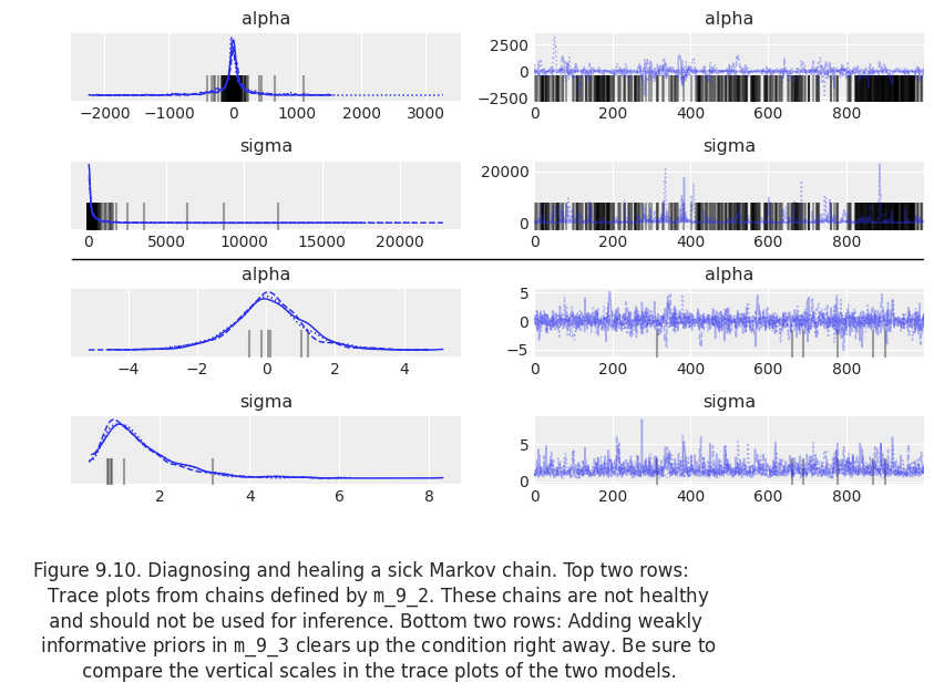
To appreciate what’s happend, let’s look at the priors (dashed) and posteriors (solid) in Figure 9.11. The Gaussian prior for \(\alpha\) and the exponential prior for \(\sigma\) contain very downhill slopes that are so gradual that even with two observations, the likelihood almost completely overcomes them. The mean of the prior for \(\alpha\) is 1 but the mean for the posterior is 0, just as the likelihood/data says it should be.
These weakly informative priors have helped provide a gentle nudge rowards reasonable values of parameters. Lots of problematic chains want subtle priors like these: Designed to tune estimations by assuming a tiny bit of prior information about each parameter. Even though the priors end up getting washed out right away as two observations were enough here, they still had a big effect on inference by allowing us to get a good answer.
Figure 9.11. Prior (dashed) and posterior (solid) for the model with weakly informative priors, m_9_3.#
# Figure 9.11
with m_9_3:
    m_9_3_prior = az.extract_dataset(
        pm.sample_prior_predictive(var_names=["alpha", "sigma"])["prior"]
    )
    m_9_3_post = az.extract_dataset(m_9_3_trace["posterior"], var_names=["alpha", "sigma"])

# _, axs = plt.subplots(1, 2, figsize=[8, 3.5], constrained_layout=True)
fig, axs = plt.subplots(1, 2, figsize=[8, 4.2], constrained_layout=True)
ax0, ax1 = axs

az.plot_kde(m_9_3_prior["alpha"].to_numpy(), ax=ax0, plot_kwargs={"color": "k", "ls": "dashed"})
az.plot_kde(m_9_3_post["alpha"].to_numpy(), ax=ax0, plot_kwargs={"color": "k"})
ax0.set_xlim(-15, 15)
ax0.set_xlabel("alpha")

az.plot_kde(
    m_9_3_prior["sigma"].to_numpy(),
    ax=ax1,
    plot_kwargs={"color": "k", "ls": "dashed"},
    label="prior",
)
az.plot_kde(m_9_3_post["sigma"].to_numpy(), ax=ax1, plot_kwargs={"color": "k"}, label="posterior")
ax1.legend()
ax1.set_xlim(0, 10)
ax1.set_xlabel("sigma")

for ax in axs:
    ax.set_ylabel("Density")

# Reserve bottom 22% of the figure for the caption before placing any text
fig.get_layout_engine().set(rect=(0, 0.22, 1, 0.78))

fig.suptitle(
    x=0.4,
    y=-0.06,
    t="Figure 9.11. Prior (dashed) and posterior (solid) for the model with weakly \n \
    informative priors, $\mathtt{m\_9\_3}$. Even with only two observations, the likelihood \n \
    easily overcomes these priors. Yet the posterior cannot be successfully  \n \
    approximated without them."
)
<>:38: SyntaxWarning: invalid escape sequence '\m'
<>:38: SyntaxWarning: invalid escape sequence '\m'
/tmp/ipykernel_825/1721737970.py:38: SyntaxWarning: invalid escape sequence '\m'
  informative priors, $\mathtt{m\_9\_3}$. Even with only two observations, the likelihood \n \
Text(0.4, -0.06, 'Figure 9.11. Prior (dashed) and posterior (solid) for the model with weakly \n informative priors, $\\mathtt{m\\_9\\_3}$. Even with only two observations, the likelihood \n easily overcomes these priors. Yet the posterior cannot be successfully \n approximated without them.')
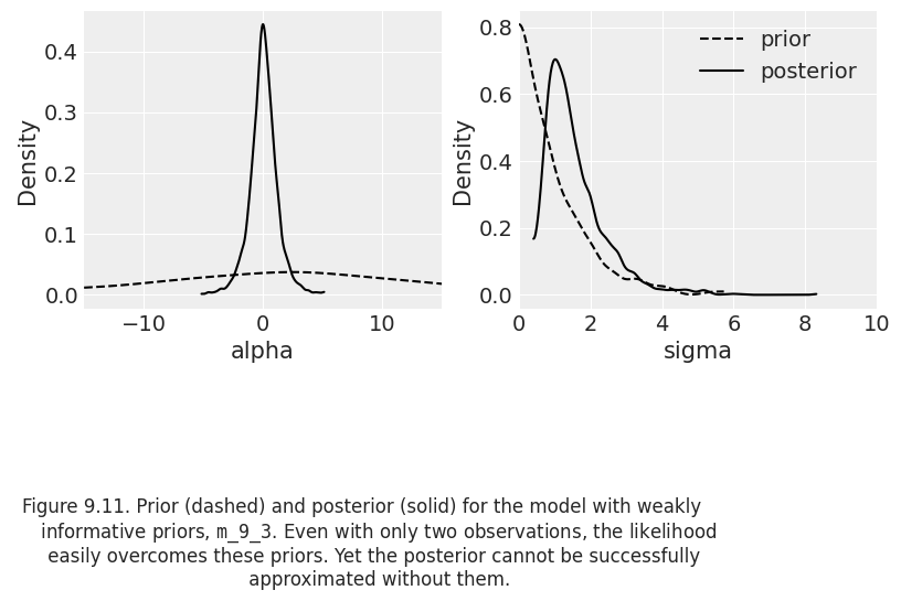
9.5.4. Non-identifiable parameters.#
Back in Chapter 5, we ran into the problem of highly correlated predictors and the non-identifiable parameters it can produce as a result. We’ll get back to this problem in this subsection by examining how they’re sampled using a Markov chain and how we can identify them by using little prior information.
Code 9.25#
First, let’s simulate 100 observations from a Gaussian distribution with a mean of 0 and a standard deviation of 1.
y = np.random.normal(loc=0, scale=1, size=100)
Code 9.26#
Next we’ll fit a model which contains two parameters that cannot be identified, \(\alpha_1\) and \(\alpha_2\). We’ll find that the posterior estimates will look suspicious with ess_bulk and r_hat values that look terrible.
We might also find that \(\alpha_1\) and \(\alpha_2\) are about the same distance from zero but on opposite sides of the spectrum.
Notice the following warning message:
ERROR:pymc.stats.convergence:There were 207 divergences after tuning. Increase `target_accept` or reparameterize.
WARNING:pymc.stats.convergence:Chain 0 reached the maximum tree depth. Increase `max_treedepth`, increase `target_accept` or reparameterize.
WARNING:pymc.stats.convergence:Chain 1 reached the maximum tree depth. Increase `max_treedepth`, increase `target_accept` or reparameterize.
ERROR:pymc.stats.convergence:The effective sample size per chain is smaller than 100 for some parameters.  A higher number is needed for reliable rhat and ess computation. See https://arxiv.org/abs/1903.08008 for details
The treedepth warnings here usually indicate inefficient chains, not necessarily broken ones. However, there’s still something seriously wrong here where if we look at the top half of Figure 9.12 on this right, you’ll see that these chains do not seem to be mixing well and are not stationary. This is a signal that these samples should not be used for inference.
with pm.Model() as m_9_4:
    a1 = pm.Normal("a1", 0, 1000)
    a2 = pm.Normal("a2", 0, 1000)

    mu = a1 + a2
    sigma = pm.Exponential("sigma", 1)

    yp = pm.Normal("y", mu, sigma, observed=y)

    m_9_4_trace = pm.sample(chains=3)

az.summary(m_9_4_trace, round_to=2)
ERROR:pymc.stats.convergence:There were 2 divergences after tuning. Increase `target_accept` or reparameterize.
WARNING:pymc.stats.convergence:Chain 0 reached the maximum tree depth. Increase `max_treedepth`, increase `target_accept` or reparameterize.
WARNING:pymc.stats.convergence:Chain 1 reached the maximum tree depth. Increase `max_treedepth`, increase `target_accept` or reparameterize.
WARNING:pymc.stats.convergence:Chain 2 reached the maximum tree depth. Increase `max_treedepth`, increase `target_accept` or reparameterize.
ERROR:pymc.stats.convergence:The effective sample size per chain is smaller than 100 for some parameters.  A higher number is needed for reliable rhat and ess computation. See https://arxiv.org/abs/1903.08008 for details
| mean | sd | hdi_5.5% | hdi_94.5% | mcse_mean | mcse_sd | ess_bulk | ess_tail | r_hat | |
|---|---|---|---|---|---|---|---|---|---|
| a1 | 23.36 | 677.01 | -807.79 | 1064.41 | 358.26 | 110.50 | 4.23 | 27.76 | 1.96 |
| a2 | -23.47 | 677.01 | -1064.49 | 807.74 | 358.26 | 110.50 | 4.23 | 27.76 | 1.96 |
| sigma | 0.90 | 0.07 | 0.78 | 1.01 | 0.01 | 0.01 | 30.74 | 50.05 | 1.10 |
# Figure 9.11 (top half)
# az.plot_trace(m_9_4_trace, figsize=[8, 4.5]);
Code 9.27#
Now the estimates for m_9_5, especially in respect to a1 and a2, are much more identified now after adding weakly informative priors. Also notice just how much faster m_9_5 was to sample as opposed to m_9_4. Bayesian statistician and godfather of modern applied Bayesian statistics, Andrew Gelman, call the problem of a model that is very slow to sample therefore being under-identified and an indication of being a bad model as folk theorem of statistical computing.
In the end, adding some weakly informative priors saves this model. Even if you think this might never apply to you, complex models can easily become unidentified given the amount of predictors, interactions, and large correlations amongst these parameters. Even having just a little prior information telling the model “none of these parameters can be 30 million” can go a long way, even if it has no effect on estimates. Note that this is different from using flat priors which shouldn’t be used.
Additionally, adding weak priors can speed up sampling because Markov chains won’t feel that it has to run out to extreme values that you, but not your model, already know are highly implausible.
with pm.Model() as m_9_5:
    a1 = pm.Normal("a1", 0, 10)
    a2 = pm.Normal("a2", 0, 10)

    mu = a1 + a2
    sigma = pm.Exponential("sigma", 1)

    yp = pm.Normal("y", mu, sigma, observed=y)

    m_9_5_trace = pm.sample(chains=3)

az.summary(m_9_5_trace, round_to=2)
| mean | sd | hdi_5.5% | hdi_94.5% | mcse_mean | mcse_sd | ess_bulk | ess_tail | r_hat | |
|---|---|---|---|---|---|---|---|---|---|
| a1 | -0.00 | 6.87 | -10.03 | 12.02 | 0.24 | 0.17 | 832.65 | 793.36 | 1.0 |
| a2 | -0.10 | 6.87 | -12.11 | 9.97 | 0.24 | 0.17 | 831.97 | 801.26 | 1.0 |
| sigma | 0.89 | 0.06 | 0.78 | 0.98 | 0.00 | 0.00 | 1259.00 | 1207.58 | 1.0 |
# Figure 9.11 (bottom half)
# az.plot_trace(m_9_5_trace, figsize=[8, 4.5]);
Figure 9.12. Same models but with weakly informative priors.#
# Figure 9.12 — combined unidentifiable vs. fixed model comparison
fig, axes = plt.subplots(6, 2, figsize=[8, 9], constrained_layout=True)

az.plot_trace(m_9_4_trace, axes=axes[0:3, :])   # unidentifiable — top half
az.plot_trace(m_9_5_trace, axes=axes[3:6, :])   # fixed          — bottom half

# Row labels
fig.text(0.005, 0.75, "m_9_4\n(flat priors)",  rotation=90, va="center", fontsize=9, weight="bold")
fig.text(0.005, 0.25, "m_9_5\n(tighter priors)", rotation=90, va="center", fontsize=9, weight="bold")

# Reserve bottom margin for the caption before computing positions
fig.get_layout_engine().set(rect=(0.03, 0.14, 1, 0.98))

# Separator line placed using the ACTUAL post-layout axes positions
top_block_bottom = axes[1, 0].get_position().y0
bottom_block_top = axes[2, 0].get_position().y1
line_y = (top_block_bottom + bottom_block_top) / 2

line = plt.Line2D([0.03, 1], [line_y, line_y],
                   transform=fig.transFigure, color="black", linewidth=1)
fig.add_artist(line)

fig.suptitle(
    x=0.4,
    y=0.03,
    t="Figure 9.12. Top panel, $\mathtt{m\_9\_4}$. A chain with wandering parameters, $\mathtt{a1}$ and $\mathtt{a2}$. \n \
    Bottom panel, $\mathtt{m\_9\_5}$. Same model but with weakly informative priors."
)
<>:26: SyntaxWarning: invalid escape sequence '\m'
<>:26: SyntaxWarning: invalid escape sequence '\m'
/tmp/ipykernel_825/1795950673.py:26: SyntaxWarning: invalid escape sequence '\m'
  t="Figure 9.12. Top panel, $\mathtt{m\_9\_4}$. A chain with wandering parameters, $\mathtt{a1}$ and $\mathtt{a2}$. \n \
Text(0.4, 0.03, 'Figure 9.12. Top panel, $\\mathtt{m\\_9\\_4}$. A chain with wandering parameters, $\\mathtt{a1}$ and $\\mathtt{a2}$. \n Bottom panel, $\\mathtt{m\\_9\\_5}$. Same model but with weakly informative priors.')
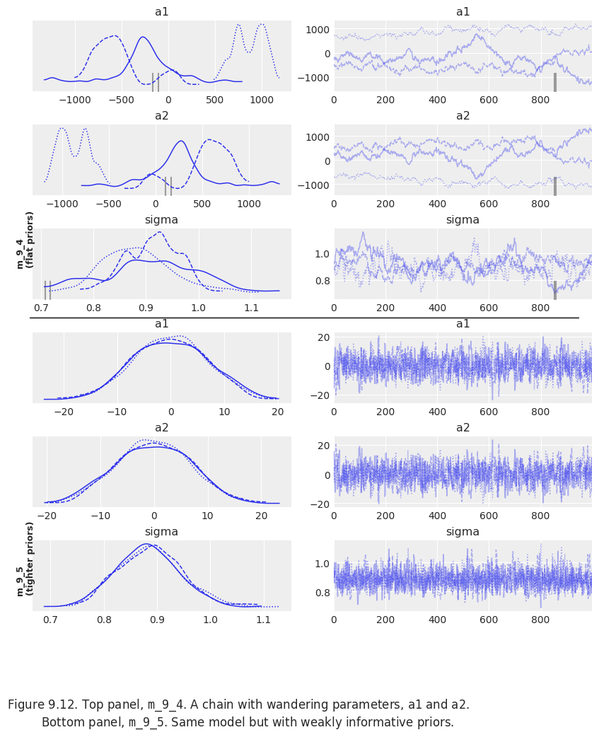
Section 9.6 - Summary#
Markov Chain Monte Carlo (MCMC) is a class of sampling algorithms, similar to others we’ve covered in previous chapters such as grid approximation and quadratic approximation, used to generate a sample from a complex, multi-dimensional probability distribution. With Bayesian models specifically, it generates a sampled approximation of the posterior distribution based on the priors distributions and likelihood/data we assign to a model but it’s impact spans far beyond just Bayesian applications, such as in statistical physics simulations, cryptographic analysis in cybersecurity, or structural biology. MCMC accomplishes this by constructing a “Markov Chain” that explores a target distribution, spending more time in areas of high probability, and uses random sampling (“Monte Carlo”) to estimate complex properties like expected values or integrals.
Markov Chain Monte Carlo was invented in the 1950’s by Stanislaw Ulam and Ed Teller with their creation of its first iteration called the Metropolis Algorithm, the oldest and simplest of the MCMC family. Just as we detailed in Section 9.1, the step-by-step explanation of the Metropolis algorithm below works the following way, assuming we’re sampling a 5x5 grid of probabilities at each cell. Note that the result is still considered to be sampled distribution even if the results can be better viewed using a heatmap, rather than a histogram, since the outcome is essentially a 25-element probability mass function spread across a spatial grid:
1. Proposal Step: Roll an eight-sided die (i.e. an octahedron dice) to propose a move in one of the following directions: 1 = North, 2 = Northeast, 3 = East, 4 = Southeast, 5 = South, 6 = Southwest, 7 = West, or 8 = Northwest.
2. Acceptance Ratio: Evaluate the posterior probability of the proposed cell \((p_{\text{move}})\) relative to the current position: $\(p_{\text{move}} = \frac{P(\text{ignition at proposed cell} \mid \text{burn pattern})}{P(\text{ignition at current position} \mid \text{burn pattern})}\)$
3. Accept/Reject Step: If \(p_{\text{move}} \geq 1\), that means the proposed cell is more probable than the current one so we can move there with certainty. If \(p_{\text{move}} < 1\), this means that the proposed cell is less probable than the current one. In this case, we then need to draw a random number (\(u\)) from a uniform random number generator between 0 and 1.
If \(u < p_{\text{move}}\), then we can move to the proposed cell. But if \(u \geq p_{\text{move}}\), then he needs stay put. The lower the ratio, the more likely the draw fails which therefore means he must stays put.
A key feature of the Metropolis algorithm is that the proposal step is symmetric since each direction has an equal chance of being proposed. Having assymetric proposals matter because there are many situations where parameters have natural constraints, such as with standard deviations where the values proposed MUST be positive. The MCMC Metropolis-Hastings algorithm improves on this limitation by adding a correction factor (\(q\)) to the acceptance ratio so that each proposal isn’t weighted equally:
Gibbs Sampling is a special case of the Metropolis-Hastings algorithm which eliminates the acceptance-rejection decision entirely and replaces it with adaptive proposals instead. What Gibbs Sampling does differently is that it updates one parameter at a time by drawing a new value directly from a conditional distribution where every other parameter constant is held constant aside from the one we’re sampling from. Because this is a direct draw from the correct distribution rather than a guess, every proposal is automatically accepted. The tradeoff with this is that the adaptive proposal is only computable for certain combinations of priors and likelihoods we can call conjugate pairs where the conditional posterior has a clean, closed-form solution to draw from directly.
However, Gibbs Sampling runs into the same scaling wall as Metropolis algorithms do where once models grow to have hundreds, or thousands, of parameters: Both algorithms still explore the posterior at one (or a few) dimension(s) at a time. In high dimensions, most of a posterior’s probability mass concentrates in a thin, curved shell far from its peak. This sampling problem is called concentration of measure where a high dimension-by-dimension sampler simply cannot navigate the sampling space efficiently since it has no sense of the posterior’s overall shape. Hamiltonian Monte Carlo solves this by using the gradient of the entire log-posterior simultaneously, letting a simulated particle roll through all dimensions at once using physics rather than blind or one-at-a-time guessing.
Here are the elements of the parable about Hamilton’s Courrier Services in section 9.3.1 that translates to how Hamiltonian Monte Carlo works conceptually:
Hamilton’s current delivery stop corresponds to the sampler’s current parameter value - his current position in the valley, north or south of town, is the one-dimensional analog of a point in parameter space. Hamilton’s location in HMC corresponds to an \(N\)th-dimension of values in a vector where each dimension represents a parameter value, such as a mean, standard deviation, y-intercept, or slope value. We can think of this vector as almost like geocoordinates within a two-dimensional space.
The valley’s shape, with the town sitting at the lowest elevation and the terrain rising toward the mountains, represents the negative log-posterior which is the potential energy surface, computed by
calc_U. The valley’s lowest point corresponds to a high posterior probability where the bulk of his customers (probability mass) actually live.The unpredictable direction and pedaling effort at the start of each leg is the random momentum draw that kicks off every HMC step.
Everything that happens afterwards, like gravity accelerating him downhill and slowing him climbing uphill, is the deterministic leapfrog simulation governed by the gradient of the posterior (
calc_U_gradient), which tells the “particle” which way is downhill at every point along its path.The moment Hamilton finally runs out of momentum and stops for a delivery is the end of a trajectory where the position gets recorded as one posterior sample before an entirely fresh random kick launches the next leg. These are the open circles in Figure 9.5.
And the low autocorrelation between his consecutive delivery stops, like where one deliver can carry him across the valley rather than shuffling to a neighbouring address, is precisely what makes HMC’s samples close to independent draws from the posterior. This is in sharp contrast to a Metropolis-style courier who only ever wanders to an adjacent block and produces a highly autocorrelated, and slow-mixing route.
In order to generate intuition about why HMC works over other approaches and when it doesn’t, let’s play with the example of a dataset with 50 \(x\) and \(y\) values each sampled from a \(\text{Normal}(0, 1)\) distribution using the example model:
\( x_i \sim \text{Normal}(\mu_x, 1)\)
\( y_i \sim \text{Normal}(\mu_y, 1)\)
\( \mu_x \sim \text{Normal}(0.05, 1)\)
\( \mu_y \sim \text{Normal}(0.05, 1)\)
(We’ll also set the the number of leapfrog steps to \(L = 11\) and the step size to \(\epsilon = 0.03\))
To initialize a sample using the MCMC Hamilton Monte Carlo algorithm, it’ll need \(5\) things to get going: two functions, two settings, and a starting point.
The first function computes the negative log-probability of the data and parameters so that the algorithm knows what the “elevation” is of a given set of parameter values at its current position. The negative log-posterior is just the negative sum of the log-likelihood of every observed data point given the current parameter values AND the log-prior density of each parameter given its own prior distribution. Once added together, we then flip the sign so that good parameter values produce low energy valleys and bad ones produce high energy hills:
\[U(\theta) = -\left[\sum_i \log P(y_i \mid \theta) + \sum_j \log P(\theta_j)\right]\]
For our specific model, our negative log-probability function looks like this:
\[ \sum_i \log p(y_i|\mu_y, 1) + \sum_i \log p(x_i|\mu_x, 1) + \log p(\mu_y|0, 0.5) + \log p(\mu_x | 0, 0.5) \]Where:
\( p(x | a, b) \) is the Gaussian density of \(x\) at mean of \(a\) and standard deviation of \(b\). So in essence, every line in our model needs to be added to one another.
# test data
np.random.seed(42)
real = stats.multivariate_normal([0, 0], np.identity(2))
x, y = real.rvs(50).T
# Q["q"] = np.array([-0.1, 0.2])

# The Negative Log-Probability
def calc_U(x, y, q, a=0, b=1, k=0, d=1):
    mu_y, mu_x = q

    U = (
        np.sum(stats.norm.logpdf(y, loc=mu_y, scale=1)) # likelihood
        + np.sum(stats.norm.logpdf(x, loc=mu_x, scale=1)) # likelihood
        + stats.norm.logpdf(mu_y, loc=a, scale=b) # prior
        + stats.norm.logpdf(mu_x, loc=k, scale=d) # prior
    )

    return -U
The second function HMC needs is a gradient of the negative log-probability (also called the loss function in ML circles) which is a separate slope measurement for each individual parameter in the model. Since we have two parameters in the model, \(\mu_x\) and \(\mu_y\), this means we’ll have two derivatives. Each one of those derivatives asks the question: “If I nudge this one parameter slightly, holding every other parameter constant, does the log-posterior increase or decrease, and how quickly?” If there’s 10 parameters in our model, we’ll get exactly 10 derivative values. Another way to express the gradient of the negative log-probability of our two parameter model is through the following equation:
\( \frac{\partial U}{\partial \mu_y} = \sum_i (y_i - \mu_y) + \frac{a - \mu_y}{b^2} \)
\(\frac{\partial U}{\partial \mu_x} = \sum_i (x_i - \mu_x) + \frac{k - \mu_x}{b^2}\)
\( \nabla U(\mu_y, \mu_x) = -\left(\frac{\partial U}{\partial \mu_y}, \ \frac{\partial U}{\partial \mu_x}\right) \)
def calc_U_gradient(x, y, q, a=0, b=1, k=0, d=1):
    mu_y, mu_x = q

    G1 = np.sum(y - mu_y) + (a - mu_y) / b**2  # dU/dmuy
    G2 = np.sum(x - mu_x) + (k - mu_x) / d**2  # dU/dmux

    return np.array([-G1, -G2])
The length of each line in Figure 9.6 is divided by the number of leapfrog steps and the step size. Leapfrog Steps (\(L\)) are simply a count of how many of the steps in your step size setting make up a full trajectory.
Step Size (\(\epsilon\)) is the distance the simulation covers in a single leapfrog set. So for example, a trajectory with \(L = 11\) and \(\epsilon = 0.03\) traces a path of roughly \(11 × 0.03 ≈ 0.33\) units long.
The problem visualized in the top-right graph of Figure 9.6 describes the U-turn Problem where a trajectory loops back onto itself because either the leapfrog steps, the step size, or both, were set too high. The No-U-Turn Sampler (NUTS) solves this problem by automatically detecting when a trajectory starts to double back on itself and stops the simulation right before that happens, rather than relying on a fixed, manually-tuned number of leapfrog steps or step size.
The following
HMC2()code ties together the two functions and settings needed to initialize our chain with a accept/rejection criterion based on the Hamiltonian dynamics of how energy was conserved in the system when simulating a particle’s trajectory:
def HMC2(U, grad_U, epsilon, L, current_q, x, y):
    q = current_q
    p = np.random.normal(loc=0, scale=1, size=len(q))  # random flick - p is momentum
    current_p = p

    # Make a half step for momentum at the beginning
    p -= epsilon * grad_U(x, y, q) / 2

    # initialize bookkeeping - saves trajectory
    qtraj = np.full((L + 1, len(q)), np.nan)
    ptraj = qtraj.copy()
    qtraj[0, :] = current_q
    ptraj[0, :] = p

    # Code 9.9 starts here
    # Alternate full steps for position and momentum
    for i in range(L):
        q += epsilon * p  # Full step for the position
        qtraj[i + 1, :] = q

        # Make a full step for the momentum, except at the end of trajectory
        if i != L - 1:
            p -= epsilon * grad_U(x, y, q)
            ptraj[i + 1, :] = p

    # Make a half step for momentum at the end
    p -= epsilon * grad_U(x, y, q) / 2
    ptraj[L, :] = p

    # Negate momentum at end of trajectory to make the proposal symmetric
    p *= -1

    # Evaluate potential and kinetic energies sat start and end of trajectory
    current_U = U(x, y, current_q)
    current_K = np.sum(current_p**2) / 2
    proposed_U = U(x, y, q)
    proposed_K = np.sum(p**2) / 2

    # Accept or reject the state at end of trajectory, returning either
    # the position at the end of the trajectory or the initial position
    accept = False

    if np.random.uniform() < np.exp(current_U - proposed_U + current_K - proposed_K):
        new_q = q  # accept
        accept = True
    else:
        new_q = current_q  # reject

    return dict(q=new_q, traj=qtraj, ptraj=ptraj, accept=accept)
The last requirement requirement for HMC is the starting point (\(q = [-0.1, 0.2]\)) which will then result in a simulation of our four trajectories, with two different leapfrog steps specified:
Q = {}
Q["q"] = np.array([-0.1, 0.2])
pr = 0.5
step = 0.03
# L = 11  # 0.03 / 28 for U-turns -- 11 for working example
n_samples = 4

_, axs = plt.subplots(1, 2, figsize=[8, 6], constrained_layout=True)

for L, ax in zip([11, 28], axs):
    ax.scatter(*Q["q"], color="k", marker="x", zorder=3)
    if L == 11:
        ax.text(*Q["q"] + 0.015, "start", weight="bold")
    for i in range(n_samples):
        Q = HMC2(U=calc_U, grad_U=calc_U_gradient, epsilon=step, L=L, current_q=Q["q"], x=x, y=y)
        ax.scatter(*Q["q"], color="w", marker="o", edgecolor="k", lw=2, zorder=3)
        if n_samples < 10:
            for j in range(L):
                K0 = np.sum(Q["ptraj"][j, :] ** 2) / 2  # kinetic energy
                ax.plot(
                    Q["traj"][j : j + 2, 0],
                    Q["traj"][j : j + 2, 1],
                    color="k",
                    lw=1 + 1 * K0,
                    alpha=0.3,
                    zorder=1,
                )
            ax.scatter(*Q["traj"].T, facecolor="w", edgecolor="gray", lw=1, zorder=2, s=10)
            if L == 11:
                ax.text(*Q["q"] + [0.02, -0.03], f"{i + 1}", weight="bold")

    ax.set_title(f"2D Gaussian, L = {L}")
    ax.set_xlabel("mux")
    ax.set_ylabel("muy")

    # draw background contours based on real probability defined above
    ax.set_xlim(-pr, pr)
    ax.set_ylim(-pr, pr)
    xs, ys = np.mgrid[-pr:pr:0.01, -pr:pr:0.01]
    p = real.logpdf(np.vstack([xs.flat, ys.flat]).T).reshape(xs.shape)
    ax.contour(xs, ys, p, 4, colors=[(0, 0, 0, 0.3)])
    ax.set_aspect(1);
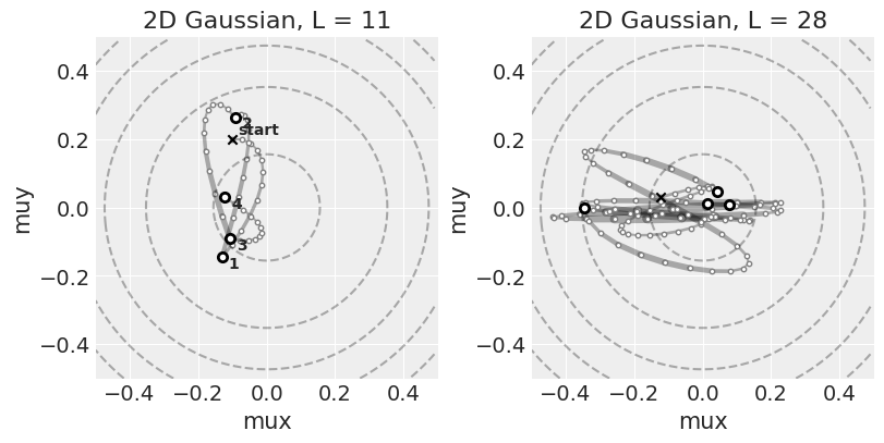
Some key evaluations metrics to watch out for using the arviz.summary() function are the following:
n_eff = ess_bulk: A crude estimate of thenumber of independent samples we got for each parameter (i.e. the effective sample size) using rank-normalized draws. This is what’s actually being estimated when we care about the reliability of the mean or median. Wheness_bulkis lower than the actual number of draws (default in PyMC is1000here but we usually set it to2000) in our chain, it means the chains are inefficient but possibly still ok.Rhat4 = r_hat: A complicated estimate of the convergence of the Markov chains to the target distribution. The Gelman-Rubin convergence diagnostic should approach1.00or more when all is well. Whenr_hatis above 1.00, it usually indicates that the chains have not yet converged so we shouldn’t trust the samples. Drawing more iterations should fix this problem. Refer to Code 9.20 to review what the 3 characteristics we should look for in a healthy trace plot using thearviz.plot_trace()` function.
Note that these diagnostics should viewed as a signal of danger but never as a signal for safety. In a situation where we have a model with extremely flat priors and little data that results in an erratic Markov chain, the solution here might be to feed it a weakly informative prior instead of flat ones.
# %load_ext watermark
# %watermark -v -iv -w