

Reverse-Engineering Hamiltonian Monte Carlo: The MCMC Engine Behind Modern Bayesian Inference#

Introduction#
The past few articles we’ve written covered the building blocks of Bayesian Inference and Statistical Machine Learning from the ground up: Starting with Bayes’ Theorem, before learning how to set up models using PyMC, then reasoning about their causal structures and the data generating processes, and using them to inform our modelling process for real data. With each Bayesian model we built, we’ve had to formally notate our prior knowledge about our parameters’ probability distributions before fitting them to our data. How the model generates a posterior distribution from our priors and likelihoods/data used to feel completely abstract. But now ‘used to’ here is the key phrase that’s a thing of the past. It’s finally clicked.
With our previous article exploring the earliest variants of the Markov Chain Monte Carlo algorithm, we’ve been able to peel back some of that abstraction. However, the mechanisms that modern probabilistic frameworks like PyMC now use have since evolved to incorporate more sophisticated techniques which means we’ll need to delve into more advanced topics this time around to develop the intuition behind them. To understand these techniques, our aim will solely be to reverse-engineer the modern descendent of MCMC that actually powers the pymc.sample() function we use to generate a posterior distribution - the Hamiltonian Monte Carlo algorithm.
The Hamiltonian Monte Carlo (HMC), for some context, is a variant of the Markov Chain Monte Carlo (MCMC) family of sampling algorithms that’s quietly running as the computational engine behind a significant share of today’s Bayesian models. Although it’s often assumed that MCMC is exclusive to Bayesian Statistics, its roots actually originate from the field of physics where it was originally developed to simulate the behaviour of the hydrogen bomb. MCMC algorithms, particularly HMC, have since had a positive impact on various diverse fields outside of Bayesian Statistics such as in epidemiology where it played a key role in modelling the effects of interventions in Europe during the spread of COVID-19 (Flaxman et al., 2020). In fact, we’ve already utilized HMC (without knowing it) in all our previous Bayesian Regression articles whenever we generated posterior distributions on total hectares burnt in a wildfire.
In this article, we’ll take a close look as to how HMC conceptually generates a posterior distribution, cover the requirements necessary to get the algorithm running, and then apply these concepts by sampling models of varying complexity. Let’s get started!
Reviewing the Metropolis-Hastings variant of MCMC#
Before we hit the ground running on Hamiltonian Monte Carlo, let’s take a step back and revisit the first iteration and the conceptual foundation of Markov Chain Monte Carlo - the Metropolis-Hastings algorithm. To quickly recap, the goal of the Metropolis-Hastings algorithm is to obtain samples from multi-dimensional probability distributions where sampling them directly is too difficult and complex. You might then ask: How then do MCMC-class algorithms avoid having to compute a highly complex, multi-dimensional distribution directly? Metropolis-Hastings, and other variants, accomplish this by constructing a random walk through parameter space where, over many draws, the visiting frequencies match the shape of the distribution they’re trying to sample from. Reviewing the basics of Metropolis-Hastings gives us the architectural foundation that HMC inherited and highlights how it resolved its past limitations. If you want a more in-depth refresher on this topic, feel free to navigate here.

Figure 1. Flowchart of the Metropolis-Hastings MCMC sampling algorithm.
Here’s the pseudocode for how the Metropolis-Hastings MCMC algorithm works:
Proposal Step: From your current position, propose a direction to move to and sample. The proposal needs to be generated randomly, such as by rolling a die.
Acceptance Ratio (\(p_{\text{move}})\): Calculate the acceptance ratio that will help determine whether the proposed position \(p(\text{proposed})\) is more, or less, likely than the current position \(p(\text{current})\):
Note that the earliest iteration of this step in 1953 assumed a symmetric proposal where the probability of proposing a move in one direction equaled the probability of proposing the reverse (i.e. a fair die). However, Professor W.K. Hastings (1970) improved this step by adding a correction factor, q, to account for asymmetric proposals which are instances where some proposals were structurally more likely than others (i.e. a loaded die). This matters in practice whenever a parameter has a natural constraint, such as with a standard deviation where its parameter values must be strictly positive.
Accept/Reject Step: If the acceptance ratio is greater than or equal to \(1\) (\(p_{move} ≥ 1\)), that means the proposed position is more probable than the current one so we can move there with certainty. And if \(p_{move} < 1\), this means the proposed position is less probable than the current one. To determine what our next move will be, we’ll need to draw a random number (\(u\)) between \(0\) and \(1\) from a uniform distribution where each number has an equal chance of being drawn:
If \(p_{move} > u\), then we can move to the proposed position. But if \(p_{move} ≤ u\), then we must stay put. The lower that \(p_{move}\) is, the more likely the draw fails which therefore means we must stay put.
Simulating Hamiltonian Mechanics#
For all innovations that Metropolis-Hastings brought to the table in terms of sampling from complex probability distributions, it wasn’t able to keep up as data and raw computational power scaled over time. Metropolis-Hastings, along with older variants of MCMC like Gibbs Sampling, hit a scaling wall when sampling from models with hundreds, let alone, thousands of parameters because it could not navigate a model’s sampling space efficiently. This was in part due to the fact that these algorithms had no sense of a posterior’s overall shape. Older variants would essentially explore a sample space blindfolded because their proposal mechanism in step 1 was random without any sense of where the high-probability regions were.
On the other hand, Hamiltonian Monte Carlo was able to overcome this limitation and sampled high-dimensional distributions more efficiently by taking advantage of their gradient information to guide its proposal mechanism. To understand how it works, we need to think of the algorithm as a simulation of a “Hamiltonian particle” that behaves similarly to a marble moving through an abstract landscape with varying peaks and valleys. However unlike a marble which will roll continuously before losing energy and eventually stopping at the lowest point due to friction, our Hamiltonian particle doesn’t have any friction to deal with. In this simulation of Hamiltonian mechanics, the particle’s trajectory also behaves like a ball being tossed in the air. During its flight upwards, gravity will slow its momentum before hitting a momentary “pause” where the ball/particle hits zero velocity at the peak of its arc before coming back down to Earth. This is exactly what happens to a Hamiltonian particle moving into a low-probability region of the landscape characterized by upward-facing slopes. The particle slows down the way a ball does climbing toward the top of its arc, and speeds back up moving into a high-probability region, the way a ball accelerates falling back toward the ground. The downward-sloping valleys in the landscape are the high probability regions.
However unlike the ball toss, a Hamiltonian particle doesn’t wait for its momentum to permanently settle to zero before we take a sample. Instead, we let the particle travel for a fixed stretch of simulated time, however far the landscape’s shape allows it to travel in that timespan, and wherever it ends up becomes the “sample” we collect for our distribution. A steep uphill section might mean the particle barely gets anywhere while a smooth downhill stretch might carry it a longer way. Either way, the sampling point isn’t chosen by the particle running out of steam, but by us.
In simpler versions of HMC, this stretch of travelling time was a fixed choice we made in advance. However as we saw with more sophisticated variants like the NUTS sampler, the algorithm instead decides this timespan adaptively during its travels. One additional detail to highlight here is that after a sample is taken, the direction of the particle’s take off, along with the force of its initial acceleration, is decided at random. However the landscape’s curvature still influences its path from that point onward.

Figure 2. Hamiltonian Monte Carlo sampling a two-dimensional probability distribution
Implementing Hamiltonian Monte Carlo#
Now that we’ve covered our simulation of the Hamiltonian particle, let’s zoom out to see how it relates to the generation of a posterior distribution from a Bayesian model and discover how each individual detail we covered plays a role in this process. To build our intuition of how Hamiltonian Monte Carlo samples a Bayesian model that’s been fitted to some data, let’s first generate a dataset with two columns of 50 random values:
import arviz as az
import matplotlib.pyplot as plt
import numpy as np
import pandas as pd
import pymc as pm
import requests
import sqlite3
import warnings

from scipy import stats
from sklearn.preprocessing import StandardScaler

warnings.simplefilter(action="ignore", category=FutureWarning)
pd.set_option("mode.chained_assignment", None)
%config Inline.figure_format = 'retina'
az.style.use("arviz-darkgrid")
az.rcParams["stats.hdi_prob"] = 0.89  # sets default credible interval used by arviz
print("Generating our test data... \n\n")

np.random.seed(42)

# test data
real = stats.multivariate_normal([0, 0], np.identity(2))
x, y = real.rvs(50).T

print(f"x (len = {len(x)}): {x}, \n\n \
y (len = {len(y)}): {y}")
Generating our test data...


x (len = 50): [ 0.49671415  0.64768854 -0.23415337  1.57921282 -0.46947439 -0.46341769
  0.24196227 -1.72491783 -1.01283112 -0.90802408  1.46564877  0.0675282
 -0.54438272 -1.15099358 -0.60063869 -0.60170661 -0.01349722  0.82254491
  0.2088636  -1.32818605  0.73846658 -0.11564828 -1.47852199 -0.46063877
  0.34361829  0.32408397 -0.676922    1.03099952 -0.83921752  0.33126343
 -0.47917424 -1.10633497  0.81252582 -0.07201012  0.36163603  0.36139561
 -0.03582604 -2.6197451   0.08704707  0.09176078 -0.21967189  1.47789404
 -0.8084936   0.91540212 -0.5297602   0.09707755 -0.70205309 -0.39210815
  0.29612028  0.00511346],

 y (len = 50): [-0.1382643   1.52302986 -0.23413696  0.76743473  0.54256004 -0.46572975
 -1.91328024 -0.56228753  0.31424733 -1.4123037  -0.2257763  -1.42474819
  0.11092259  0.37569802 -0.29169375  1.85227818 -1.05771093 -1.22084365
 -1.95967012  0.19686124  0.17136828 -0.3011037  -0.71984421  1.05712223
 -1.76304016 -0.38508228  0.61167629  0.93128012 -0.30921238  0.97554513
 -0.18565898 -1.19620662  1.35624003  1.0035329  -0.64511975  1.53803657
  1.56464366  0.8219025  -0.29900735 -1.98756891  0.35711257 -0.51827022
 -0.50175704  0.32875111  0.51326743  0.96864499 -0.32766215 -1.46351495
  0.26105527 -0.23458713]
1.Negative Log-Posterior function.#
Going back to our simulation, the geometric landscape that influences where the Hamiltonian particle is more likely to travel is calculated based on the model we’re sampling from. Notice how Figure 2 illustrates the movement of the particle in a two-dimensional landscape? To put it simply, each parameter in a model actually represents a dimension of that landscape. Although it’s not possible for us to visualize how this process works with a hundred parameter model, we can be confident that the principles for the Hamiltonian particle’s motion remain the same regardless of its landscape’s dimension size. To compute the landscape for our Hamiltonian particle to traverse through, we need to write what’s called a negative log-posterior function. The purpose of the negative log-posterior function is to compute the negative log-probability of the data and its parameters so that the algorithm knows what the “elevation” is for a given set of values at that position. For some that might have been a mouthful so let’s take a step back. Think of every possible combination of parameter values as a point in a landscape, where the number of dimensions equals the number of parameters in your model. With our synthetic dataset, our model has exactly two parameters, \(\mu_x\) and \(\mu_y\), so we can think of the particle’s position as an \(xy\)-coordinate pair (\(\mu_x\), \(\mu_y\)), in a two-dimensional space. Now the way to calculate the negative log-posterior (also known as the loss function in machine learning circles), regardless of the dimension size or parameter count, is simply to sum the log-likelihood of every observed data point given the current parameter values AND the log-prior density of each parameter given its own prior distribution. Once our mathematical equation has returned a sum, we then flip the sign so that the good parameter values produce low energy (high probability) valleys while the bad ones produce high energy (low probability) hills:
\(U(\theta) = -\left[\sum_i \log P(y_i \mid \theta) + \sum_j \log P(\theta_j)\right]\)
Now if we take our generic model from earlier, the negative log-probability function will look like the following where essentially each line in the model is added together. Notice how the first two terms on the left are summed across every data point (as per our rule above) since these represent the log-likelihood of our data, given the current parameters. On the other hand, the last two appear only once each since there’s just a single \(\mu_x\) and \(\mu_y\) shared across the whole dataset:
\(U(\theta) = -\left[\sum_i \log p(y_i|\mu_y, 1) + \sum_i \log p(x_i|\mu_x, 1) + \log p(\mu_y|0, 0.5) + \log p(\mu_x | 0, 0.5)\right]\)
And here’s the code form of that equation:
# The Negative Log-Probability
def calc_U(q, x, y, a=0, b=0.5, k=0, d=0.5):
    mu_y, mu_x = q
    U = (
        np.sum(stats.norm.logpdf(y, loc=mu_y, scale=1)) # likelihood
        + np.sum(stats.norm.logpdf(x, loc=mu_x, scale=1)) # likelihood
        + stats.norm.logpdf(mu_y, loc=a, scale=b) # prior
        + stats.norm.logpdf(mu_x, loc=k, scale=d) # prior
    )
    return -U
Great, so hopefully we understand how the “landscape” for our Hamiltonian particle is generated based on a simple model. Now, what does this calc_U() function look like if we’re having to sample from a significantly more complicated one? Let’s test that by bringing back a revamped version of our old Multiple Linear Regression that we used to model wildfire size but instead, we’ll upgrade it to a Hierarchical Multi-Level Regression model!
\(Where:\)
\(W_i, L_i, Pn_i, T_i, R_i, H_i\) correspond to
wind_speed,lightning,person,temp,precip, andvpdrespectively.
#######################
### DATA EXTRACTION ###
#######################
db_link = "https://raw.githubusercontent.com/vanislekahuna/wps-labs/main/data/historical_bc_wildfires/bc_wildfires.db"
response = requests.get(db_link)
with open("bc_wildfires.db", "wb") as f:
    f.write(response.content)

conn = sqlite3.connect('bc_wildfires.db')
cursor = conn.cursor()

join_query = """
WITH weather AS (
    SELECT wind_speed_ms, wind_direction_deg, wind_direction, temperature_c AS temp_c_ign_date, humidity_dewpoint_temperature_2m AS humidity_dewpoint_temp_k_ign_date, soil_temperature_level_1 AS soil_temp_lvl1_ign_date, fire_label AS weather_fire_label
    FROM weather_data
),
terraclimate AS (
    SELECT monthly_mean_temp_c, monthly_total_precip_mm, monthly_mean_humidity_vpd_kPa, monthly_mean_soil_moisture_mm, fire_label AS terraclimate_fire_label
    FROM terraclimate_bc_weather
)
SELECT *
FROM historical_bc_wildfires
LEFT JOIN weather ON historical_bc_wildfires.FIRELABEL = weather.weather_fire_label
LEFT JOIN terraclimate ON historical_bc_wildfires.FIRELABEL = terraclimate.terraclimate_fire_label
WHERE historical_bc_wildfires.SIZE_HA IS NOT NULL
AND historical_bc_wildfires.SIZE_HA > 0
AND historical_bc_wildfires.FIRELABEL NOT IN ('1951-R00037', '1951-R00050', '1951-R00060', '1951-R00067', '1951-R00069', '1951-R00070', '1956-R00107', '1958-V00283', '1956-R00160', '1968-R00088', '1985-V70083', '1985-V70088', '1987-V90016', '1990-V50012');
"""

df = pd.read_sql_query(join_query, conn)


wildfire_df = df[
    [
        "FRCNTR",
        "FIRELABEL",
        "IGN_DATE",
        "FIRE_CAUSE",
        "SIZE_HA",
        "wind_speed_ms",
        "temp_c_ign_date",
        "humidity_dewpoint_temp_k_ign_date",
        "soil_temp_lvl1_ign_date",
        "monthly_mean_temp_c",
        "monthly_total_precip_mm",
        "monthly_mean_humidity_vpd_kPa",
        "monthly_mean_soil_moisture_mm"
    ]
  ].copy()

print(f"wildfire_df shape: {wildfire_df.shape} \n")
wildfire_df shape: (162905, 13)
###########################
### DATA TRANSFORMATION ###
###########################
centres = wildfire_df["FRCNTR"].unique()

wildfire_df["size_log1ptransformed"] = np.log1p(wildfire_df["SIZE_HA"])
wildfire_df["wind_speed_log1ptransformed"] = np.log1p(wildfire_df["wind_speed_ms"])
wildfire_df["soil_temp_c_lvl1_ign_date"] = wildfire_df["soil_temp_lvl1_ign_date"] - 273.15

one_hot_encodding = pd.get_dummies(wildfire_df["FIRE_CAUSE"], dtype=int)

wildfire_df = pd.concat([wildfire_df, one_hot_encodding], axis=1)

large_fire_df = wildfire_df[wildfire_df['SIZE_HA'] >= 100].dropna()

print(f"\n large_fire_df shape: {large_fire_df.shape} \n")
large_fire_df shape: (3818, 19)
###################################
### DATA LOADING/PRE-PROCESSING ###
###################################
continuous_cols = ["wind_speed_log1ptransformed", "temp_c_ign_date",
                    "monthly_total_precip_mm", "monthly_mean_humidity_vpd_kPa"]
X_cont_std = StandardScaler().fit_transform(large_fire_df[continuous_cols])

X_mat = np.column_stack([
    X_cont_std[:, 0],
    large_fire_df["Lightning"].values,
    large_fire_df["Person"].values,
    X_cont_std[:, 1],
    X_cont_std[:, 2],
    X_cont_std[:, 3],
])

zone_labels = sorted(large_fire_df["FRCNTR"].astype(str).unique())
zone_to_idx = {z: i for i, z in enumerate(zone_labels)}
zone_idx = large_fire_df["FRCNTR"].astype(str).map(zone_to_idx).values
print(f"Value count of generated zone labels: \n{pd.Series(zone_idx).value_counts().sort_index()}")

y = large_fire_df["size_log1ptransformed"].values
Value count of generated zone labels:
0     343
1     406
2    1327
3     591
4     651
5     500
Name: count, dtype: int64
##############################################################
### HIERARCHICAL MULTI-LEVEL BAYESIAN REGRESSION MODELLING ###
##############################################################
coords = {
    "zone": zone_labels,
    "predictor": ["wind_speed", "lightning", "person", "temp", "precip", "vpd"],
    "obs_id": np.arange(len(y)),
}

with pm.Model(coords=coords) as hier_model:

    zone_idx_ = pm.Data("zone_idx", zone_idx, dims="obs_id")
    X = pm.Data("X_mat", X_mat, dims=("obs_id", "predictor"))

    # Population-level (grand mean across zones)
    mu_alpha = pm.Normal("mu_alpha", mu=4.0, sigma=0.5)      # log(100+1) ≈ 4.6, our size floor
    mu_beta  = pm.Normal("mu_beta", mu=0.0, sigma=1.0, dims="predictor")

    # Between-zone SD — magnitude of cross-zone heterogeneity per effect
    sigma_alpha = pm.HalfNormal("sigma_alpha", sigma=0.5)
    sigma_beta  = pm.HalfNormal("sigma_beta", sigma=0.5, dims="predictor")

    # Non-centered parameterization
    z_alpha = pm.Normal("z_alpha", 0.0, 1.0, dims="zone")
    z_beta  = pm.Normal("z_beta", 0.0, 1.0, dims=("zone", "predictor"))

    alpha_zone = pm.Deterministic("alpha_zone", mu_alpha + sigma_alpha * z_alpha, dims="zone")
    beta_zone  = pm.Deterministic("beta_zone", mu_beta + sigma_beta * z_beta, dims=("zone", "predictor"))

    mu = alpha_zone[zone_idx_] + (beta_zone[zone_idx_] * X).sum(axis=-1)

    sigma_y = pm.HalfNormal("sigma_y", sigma=0.5)
    y_obs = pm.Normal("y_obs", mu=mu, sigma=sigma_y, observed=y, dims="obs_id")


    idata = pm.sample(
        draws=2000,
        tune=2000,
        chains=4,
        target_accept=0.95,   # higher than default — hierarchical funnels need this
        random_seed=42,
        idata_kwargs={"log_likelihood": True},  # needed for LOO below
    )


n_div = idata.sample_stats["diverging"].sum().item()
print(f"Divergences: {n_div}")

az.summary(idata, var_names=["mu_alpha", "mu_beta", "sigma_alpha", "sigma_beta", "sigma_y"])
Divergences: 0
| mean | sd | hdi_5.5% | hdi_94.5% | mcse_mean | mcse_sd | ess_bulk | ess_tail | r_hat | |
|---|---|---|---|---|---|---|---|---|---|
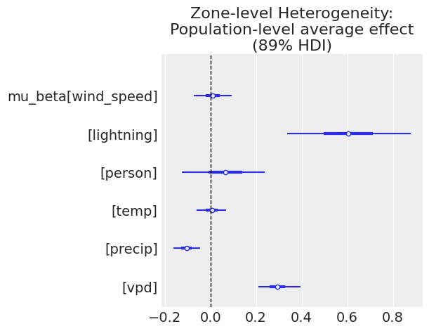
| mu_alpha | 5.619 | 0.316 | 5.136 | 6.084 | 0.006 | 0.005 | 3191.0 | 4539.0 | 1.0 |
| mu_beta[wind_speed] | 0.011 | 0.058 | -0.074 | 0.093 | 0.001 | 0.002 | 4272.0 | 3963.0 | 1.0 |
| mu_beta[lightning] | 0.602 | 0.174 | 0.337 | 0.878 | 0.002 | 0.003 | 5432.0 | 5526.0 | 1.0 |
| mu_beta[person] | 0.067 | 0.116 | -0.127 | 0.238 | 0.001 | 0.002 | 8065.0 | 5421.0 | 1.0 |
| mu_beta[temp] | 0.004 | 0.044 | -0.060 | 0.069 | 0.001 | 0.001 | 6615.0 | 4902.0 | 1.0 |
| mu_beta[precip] | -0.107 | 0.040 | -0.164 | -0.044 | 0.001 | 0.001 | 6599.0 | 4260.0 | 1.0 |
| mu_beta[vpd] | 0.295 | 0.061 | 0.210 | 0.394 | 0.001 | 0.001 | 5417.0 | 4780.0 | 1.0 |
| sigma_alpha | 0.553 | 0.238 | 0.224 | 0.907 | 0.004 | 0.003 | 3582.0 | 5259.0 | 1.0 |
| sigma_beta[wind_speed] | 0.102 | 0.072 | 0.000 | 0.181 | 0.001 | 0.002 | 2303.0 | 2901.0 | 1.0 |
| sigma_beta[lightning] | 0.317 | 0.143 | 0.113 | 0.519 | 0.002 | 0.002 | 4364.0 | 3612.0 | 1.0 |
| sigma_beta[person] | 0.104 | 0.094 | 0.000 | 0.214 | 0.001 | 0.002 | 4270.0 | 4186.0 | 1.0 |
| sigma_beta[temp] | 0.055 | 0.051 | 0.000 | 0.112 | 0.001 | 0.001 | 3663.0 | 4551.0 | 1.0 |
| sigma_beta[precip] | 0.056 | 0.049 | 0.000 | 0.111 | 0.001 | 0.001 | 3373.0 | 4503.0 | 1.0 |
| sigma_beta[vpd] | 0.098 | 0.076 | 0.000 | 0.186 | 0.001 | 0.002 | 2543.0 | 3732.0 | 1.0 |
| sigma_y | 1.378 | 0.016 | 1.354 | 1.405 | 0.000 | 0.000 | 12740.0 | 5707.0 | 1.0 |
# ZONE-LEVEL HETEROGENEITY:
# Population-level average effect (across all zones)
az.plot_forest(idata, var_names=["mu_beta"], combined=True, hdi_prob=0.89)
plt.axvline(0, color='black', linestyle='--', linewidth=1)
plt.title("Zone-level Heterogeneity: Population-level average effect (89% HDI)")
Text(0.5, 1.0, 'Zone-level Heterogeneity: Population-level average effect (89% HDI)')
# ZONE-LEVEL HETEROGENEITY:
# Zone-specific coefficients, partially pooled
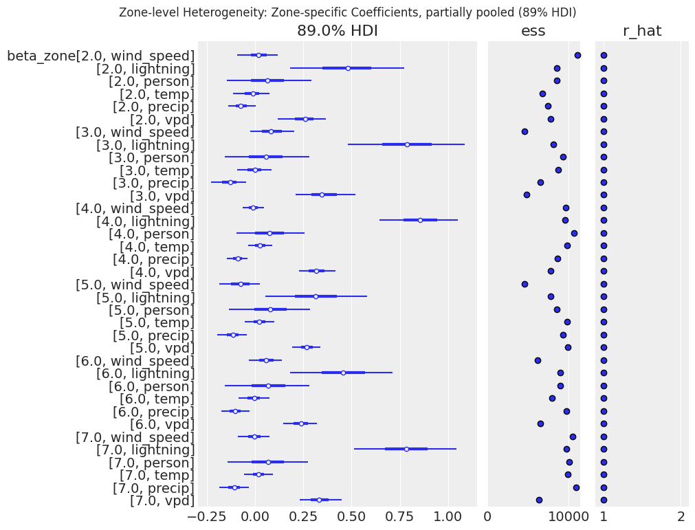
az.plot_forest(idata, var_names=["beta_zone"], combined=True, r_hat=True, ess=True)
plt.gcf().suptitle("Zone-level Heterogeneity: Zone-specific Coefficients, partially pooled (89% HDI)")
Text(0.5, 0.98, 'Zone-level Heterogeneity: Zone-specific Coefficients, partially pooled (89% HDI)')
# POSTERIOR PREDICTIVE CHECK
with hier_model:
    hierarchical_model_ppc = pm.sample_posterior_predictive(idata, random_seed=42)
    idata.extend(hierarchical_model_ppc)

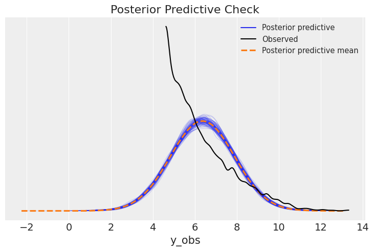
az.plot_ppc(idata, num_pp_samples=100)
plt.title("Posterior Predictive Check")
Text(0.5, 1.0, 'Posterior Predictive Check')
# PREDICTIVE PREFORMANCE: Bayesian R² (Gelman et al. 2019 formulation)
y_pred_samples = idata.posterior_predictive["y_obs"].values.reshape(-1, len(y))
bayes_r2 = az.r2_score(y, y_pred_samples)
print(bayes_r2)


# LOO — The natural comparison point against a non-hierarchical (complete-pooling) version of this same model to formally test whether the hierarchy earns its added complexity
loo = az.loo(idata, pointwise=True)
print(loo)

high_k = (loo.pareto_k.values > 0.7).sum()
print(f"Observations with unreliable LOO estimates: {high_k}")
r2        0.368264
r2_std    0.005967
dtype: float64
Computed from 8000 posterior samples and 3818 observations log-likelihood matrix.

         Estimate       SE
elpd_loo -6658.65    51.09
p_loo       26.64        -
------

Pareto k diagnostic values:
                         Count   Pct.
(-Inf, 0.70]   (good)     3818  100.0%
   (0.70, 1]   (bad)         0    0.0%
   (1, Inf)   (very bad)    0    0.0%

Observations with unreliable LOO estimates: 0
With the following equation + code, the important piece here is not to get stuck on the technical complexity of the model itself but instead on the position of each parameter, whether that’s the prior or the likelihood. The take-home point here is that regardless of our model’s complexity, the elevation at any given point in our Hamiltonian particle’s landscape is essentially just a sum of log-probability contributions from every one of its parameters:
$ \sum_i \log p(y_i \mid \mu_i, \sigma_y) + \log p(\mu_\alpha \mid 4, 0.5) + \sum_p \log p(\mu_{\beta,p} \mid 0, 1) + \log p(\sigma_\alpha \mid 0, 0.5) \
\sum_p \log p(\sigma_{\beta,p} \mid 0, 0.5) + \sum_j \log p(z_{\alpha,j} \mid 0, 1) + \sum_{j,p} \log p(z_{\beta,j,p} \mid 0, 1) + \log p(\sigma_y \mid 0, 0.5) $
def unpack_params(q, J, P):
    """
    Slice a flat parameter vector q into its named pieces. This mirrors
    what PyTensor does internally inside PyMC -- every model, no matter
    how many groups or predictors it has, ultimately reduces to one long
    vector that the sampler walks through.
    """
    idx = 0
    mu_alpha    = q[idx]; idx += 1
    mu_beta     = q[idx:idx+P]; idx += P
    sigma_alpha = q[idx]; idx += 1
    sigma_beta  = q[idx:idx+P]; idx += P
    z_alpha     = q[idx:idx+J]; idx += J
    z_beta      = q[idx:idx+J*P].reshape(J, P); idx += J*P
    sigma_y     = q[idx]; idx += 1
    return mu_alpha, mu_beta, sigma_alpha, sigma_beta, z_alpha, z_beta, sigma_y


def hierarchical_calc_U(q, X, y, zone_idx, J, P,
           mu_alpha_prior=(4.0, 0.5), mu_beta_prior=(0.0, 1.0),
           sigma_alpha_prior=0.5, sigma_beta_prior=0.5, sigma_y_prior=0.5):
    """Negative log-posterior (potential energy) at a single point q."""
    mu_alpha, mu_beta, sigma_alpha, sigma_beta, z_alpha, z_beta, sigma_y = \
        unpack_params(q, J, P)

    # HalfNormal parameters have zero density outside their support.
    # Real NUTS avoids this entirely by sampling on a log-transformed, constrained scale internally.
    # We stay on the natural scale here.
    if sigma_alpha <= 0 or np.any(sigma_beta <= 0) or sigma_y <= 0:
        return np.inf

    # Non-centered transform (matches the pm.Deterministic lines)
    alpha_zone = mu_alpha + sigma_alpha * z_alpha
    beta_zone  = mu_beta + sigma_beta * z_beta

    # Linear predictor
    mu = alpha_zone[zone_idx] + np.sum(beta_zone[zone_idx] * X, axis=-1)

    log_lik = np.sum(stats.norm.logpdf(y, loc=mu, scale=sigma_y))

    log_prior = (
        stats.norm.logpdf(mu_alpha, *mu_alpha_prior)
        + np.sum(stats.norm.logpdf(mu_beta, *mu_beta_prior)) # one sum per predictor - 6 predictors (6 parameters)
        + stats.halfnorm.logpdf(sigma_alpha, scale=sigma_alpha_prior)
        + np.sum(stats.halfnorm.logpdf(sigma_beta, scale=sigma_beta_prior)) # one sum per predictor - 6 predictors (6 parameters)
        + np.sum(stats.norm.logpdf(z_alpha, 0.0, 1.0)) # one sum per zone - 6 zones (6 parameters)
        + np.sum(stats.norm.logpdf(z_beta, 0.0, 1.0)) # one sum per zone per predictor - 6 zones x 6 predictors (36 parameters)
        + stats.halfnorm.logpdf(sigma_y, scale=sigma_y_prior)
    )

    return -(log_lik + log_prior)
2.Gradient of the Negative Log Probability function.#
The second function that the Hamiltonian Monte Carlo algorithm needs is the gradient of the negative log-probability which is a separate slope measurement for each individual parameter in the model. Going back to our Hamiltonian mechanics simulation, the element there that represents the gradient of the negative log probability is the force acting on the particle at its current location. If we’re reusing the ball toss analogy, the gradient here is functioning as the gravity in the toss. For contrast, while the negative log-probability function is calculating the shape of the landscape and determining where the peaks and valleys are, the gradients add value by acting as the “gravity” force in the simulation. However, unlike real-life gravity where its strength remains constant, the gravity of the gradient in the Hamiltonian mechanics simulation varies by location. The pull is strongest in the steepest terrains and essentially non-existent on flat surfaces. Now coming back to our simple model, since we only have two parameters in the model, \(\mu_x\) and \(\mu_y\), this means we’ll only have two derivatives to account for. Each one of those derivatives asks the question: “If I nudge this one parameter slightly, holding every other parameter constant, does the log-posterior increase or decrease, and how quickly?” If there’s 10 parameters in our model, we’ll get exactly 10 derivative values. However as our model grows more structured and complex, such as in the case with our hierarchical wildfire model, some of those derivatives need an extra chain-rule step to account for how one parameter influences another. So for simplicity’s sake, we’ll stick with the simple model for the rest of this overview. To express the gradient of the negative log-probability for our two parameter model, we’ll use the following equation:
\( \frac{\partial U}{\partial \mu_y} = \sum_i (y_i - \mu_y) + \frac{a - \mu_y}{b^2} \)
\(\frac{\partial U}{\partial \mu_x} = \sum_i (x_i - \mu_x) + \frac{k - \mu_x}{d^2}\)
\( \nabla U(\mu_y, \mu_x) = -\left(\frac{\partial U}{\partial \mu_y}, \ \frac{\partial U}{\partial \mu_x}\right) \)
And the associated Python function for this specific, two-parameter model gradient would be:
# Gradient of the Negative Log-Probability
def calc_U_gradient(q, x, y, a=0, b=0.5, k=0, d=0.5):
    mu_y, mu_x = q

    G1 = np.sum(y - mu_y) + (a - mu_y) / b**2  # dU/dmuy
    G2 = np.sum(x - mu_x) + (k - mu_x) / d**2  # dU/dmux

    return np.array([-G1, -G2])
3.Leapfrog Steps (\(L\)).#
Ok, now that we’ve covered the most complex parts of HMC with the functions, let’s quickly cover the two settings we need to tune in order to get the algorithm started. The first is the leapfrog steps (\(L\)) which is simply the count of how many steps our Hamiltonian particle takes to complete one trajectory. If you remember earlier in the ball toss analogy, we mentioned how we specify the span of time that the ball spends in the air? Together, these two settings determine how long our particle’s trajectory runs before we stop and record a sample.
4.Step Size (ϵ).#
The second setting we need to tune is the step size (ϵ) which is the distance the simulation covers in a single leapfrog set. For example with our simple model notation from earlier, we specified that: “The number of leapfrog steps to \(L = 11\) and the step size to \(ϵ = 0.03\).” With the leapfrog step and step size specified, a trajectory with \(L = 11\) and \(ϵ = 0.03\) traces a path of roughly \(11 × 0.03 ≈ 0.33\) units long.
An issue that may arise from these two settings is that if we specify a poor combination of the leapfrog steps and the step size then we can run into an issue known as the U-turn problem. The U-turn problem arises when a Hamiltonian particle’s simulated trajectory travels far enough to loop back to its own starting point or the general area it started from. As a consequence of this issue, we’ll end up with consecutive samples that are highly autocorrelated and will require far more computation for the particle to explore its landscape.
Luckily, Hoffman and Gelman (2014) solved this problem over a decade ago now with their proposal of the No-U-Turn Sampler (NUTS). In essence, what the No-U-Turn Sampler (NUTS) does is automatically detect when a trajectory starts to double back on itself and stops the simulation right before that happens, instead of relying on a fixed, manually-tuned number of leapfrog steps (\(L\)) or step size (\(ϵ\)) settings. By now, many sophisticated probabilistic programming tools like PyMC have widely adopted the NUTS sampler to generate distributions of continuous variables.
5.Starting Point.#
The last requirement for HMC is the starting point which we’ll arbitrarily assign to (\(q = [-0.1, 0.2]\)). The starting point will kick off our “Hamiltonian particle” simulation which allows us to sample from a posterior distribution based on which areas the particle visits most frequently. Once we plug in our two functions and two settings, with the flexibility to plug in whichever model’s functions we’re sampling from, then our entire Hamiltonian Monte Carlo sampler will look like the following:
def Hamiltonian_Monte_Carlo(U, grad_U, epsilon, L, current_q, *args):
    q = current_q.copy()
    p = np.random.normal(loc=0, scale=1, size=len(q))  # random flick - p is momentum
    current_p = p.copy()

    # Make a half step for momentum at the beginning
    p -= epsilon * grad_U(q, *args) / 2

    # initialize bookkeeping - saves trajectory
    qtraj = np.full((L + 1, len(q)), np.nan)
    ptraj = qtraj.copy()
    qtraj[0, :] = current_q
    ptraj[0, :] = p

    # Code 9.9 starts here
    # Alternate full steps for position and momentum
    for i in range(L):
        q += epsilon * p  # Full step for the position
        qtraj[i + 1, :] = q

        # Make a full step for the momentum, except at the end of trajectory
        if i != L - 1:
            p -= epsilon * grad_U(q, *args)
            ptraj[i + 1, :] = p

    # Make a half step for momentum at the end
    p -= epsilon * grad_U(q, *args) / 2
    ptraj[L, :] = p

    # Negate momentum at end of trajectory to make the proposal symmetric
    p *= -1

    # Evaluate potential and kinetic energies at start and end of trajectory
    current_U = U(current_q, *args)
    current_K = np.sum(current_p**2) / 2
    proposed_U = U(q, *args)
    proposed_K = np.sum(p**2) / 2

    # Accept or reject the state at end of trajectory, returning either
    # the position at the end of the trajectory or the initial position
    accept = False

    if np.random.uniform() < np.exp(current_U - proposed_U + current_K - proposed_K):
        new_q = q  # accept
        accept = True
    else:
        new_q = current_q  # reject

    return dict(q=new_q, traj=qtraj, ptraj=ptraj, accept=accept)
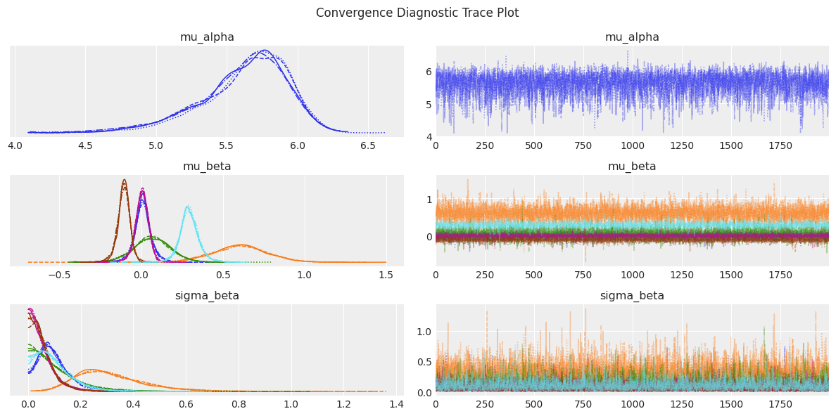
And often one of the results we like to see immediately after running the sampler is a trace plot to evaluate its preformance. With a healthy trace plot, we generally want to see two things. The first thing to look for within each individual chain is that the particle should fluctuate rapidly and densely around a stable value, not drift steadily upward or downward over time. The second thing to look for across all four chains is that all four chains should converge on that same stable value. Chains that settle into visibly different regions signal a problem, even if each one looks stable on its own. The trace plot below is an example of a high preforming chain that was generated for the complex Hierarchical Bayesian Regression from earlier.
az.plot_trace(idata, var_names=["mu_alpha", "mu_beta", "sigma_beta"], compact=True)
plt.gcf().suptitle("Convergence Diagnostic Trace Plot")
plt.tight_layout()
/tmp/ipykernel_2906/3113986826.py:3: UserWarning: The figure layout has changed to tight
  plt.tight_layout()
Closing Thoughts#
We set out to reverse-engineer the machine behind modern Bayesian inference and by now, we’ve succeeded in taking it apart! Let’s recap what we accomplished. What began as an abstract black box that somehow turned priors and likelihoods into a posterior distribution is a black box no longer. We then traced the lineage from Metropolis-Hastings’ blind, random walk through parameter space, to the moment gradient information transformed that walk into something far more deliberate: A Hamiltonian particle, gliding through a landscape shaped by our own model’s mathematics, accelerating into high-probability valleys and decelerating up low-probability slopes. Lastly, we built the two functions that define that landscape and the forces acting on it, tuned the two settings that govern how far our particle travels, and watched all five pieces come together into a single, working sampler.
What makes this worth understanding isn’t just the mechanics themselves: It’s the foundation with which we’re using Bayesian Inference to drive real-world impact. Every time pymc.sample() runs, this sophisticated, and highly robust, simulation of a “Hamiltonian particle” is what’s quietly happening underneath it all. Hamiltonian Monte Carlo isn’t a niche statistical curiosity but rather, the quiet computational engine behind a significant share of the inference done in Bayesian statistics today. For example, we noted in the intro how it played a direct role in modeling the effects of interventions across Europe during COVID-19 which helped shape real public health decisions during a genuine crisis (Flaxman et al., 2020).
We even saw its reach firsthand, too. The same skeleton that generated a posterior distribution for a toy two-parameter model was able to scale, without needing to be reinvented, to a complex Hierarchical Bayesian Regression model spanning dozens of parameters across BC’s Fire Centre zones. With our HMC quietly working in the background, our Hierarchical Bayesian Regression model was able to estimate how wind speed, lightning, precipitation, and a handful of other atmospheric variables could shape the size of a BC wildfire, with the uncertainty in that estimate quantified honestly rather than papered over. Our toy example of HMC scaled to a complex machine running on real data, producing a real answer to a real question!
We came into this article treating the posterior as something that simply appeared. Now we can now proudly say we’re leaving it with a working understanding of exactly how it gets there though one leapfrog step, one gradient, and one accepted proposal at a time.
Thank you for reading through to the very end. This was an amazing journey I’m glad we were able to travel through together.
References#
Flaxman, S., Mishra, S., Gandy, A., Unwin, H. J. T., Mellan, T. A., Coupland, H., … & Bhatt, S. (2020). Estimating the effects of non-pharmaceutical interventions on COVID-19 in Europe. Nature, 584(7820): 257-261. https://www.nature.com/articles/s41586-020-2405-7
Hastings, W.K. (1970). Monte Carlo Sampling Methods Using Markov Chains and Their Applications. Biometrika. 57(1): 97–109. https://bpb-us-e1.wpmucdn.com/sites.psu.edu/dist/d/175237/files/2023/12/Hastings1970_Murali-Haran.pdf
Hoffman, M. D., & Gelman, A. (2014). The No-U-Turn sampler: adaptively setting path lengths in Hamiltonian Monte Carlo. J. Mach. Learn. Res., 15(1), 1593-1623. https://arxiv.org/pdf/1111.4246
McElreath, R. (2020). Statistical Rethinking: A Bayesian Course with examples in R and Stan. Routledge.